How to simulate a population RMSEA in Structural Equation Modelling?

Anyone who has ever done any Structural Equation Modelling (SEM) analyses knows that, sooner or later, you will need to work with fit indices. Not everybody likes them (some people will be forever hooked on the chi-square test of fit), but it is pretty safe to say that, nowadays, if you have good approximate fit your model is good enough to be published. One thing that not everybody takes the time to think about though is the fact that these numbers can be thought of as estimates of population fit indices.

One of the (MANY) reasons of why people like Steiger & Lindt’s Root Mean Square Error (RMSEA) is because (aside from being a sensible number to calculate) it has a population definition and a sampling distribution that is theoretically known. And, as it always happen, if you know the sampling distribution of the test statistic you can perform some type of inference on it. For the case of the RMSEA, Steiger defined the population RMSEA as:

$RMSEA = \sqrt \frac{F}{df}$

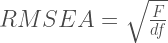
Where F is the minimum of the fit function when the (misspecified) model is applied to the population covariance matrix and ‘df’ is the degrees of freedom of the model.

When you can simulate data where the RMSEA value is known in the population, you can start make a lot of sensible claims about stuff like power or bias regarding the characteristics of your data. But, how do you simulate data where you know the population value of the RMSEA ahead of time? Well, curiously enough it is surprisingly simple. All you need to know is the population covariance matrix and a misspecified model that you would fit to it. As usual, this example will be demonstrated in the R package lavaan because lavaan is pretty awesome.

The first thing we’re going to do is we’re gonna come up with some factor model that we’re going to transform into a population covariance matrix. So, in this case, I’m choosing a 3 factor model with equal loadings of 0.7, factor correlations of 0.5 and factor variances fixed at 1. Or, in code, it would look like this:

mod1 <- 'f1 =~ 0.7*y1 + 0.7*y2 +0.7*y3 +0.7*y4 f2 =~ 0.7*y5 + 0.7*y6 +0.7*y7 +0.7*y8 f3 =~ 0.7*y9 + 0.7*y10 +0.7*y11 +0.7*y12
f1 ~~ 0.5*f2 f1 ~~ 0.5*f3 f2 ~~ 0.5*f3

f1 ~~ 1*f1 f2 ~~ 1*f2 f3 ~~ 1*f3'
dat1 <- simulateData(mod1,1, meanstructure=FALSE, return.fit=TRUE) pop.sigm <- fitted(attr(dat1, 'fit'))$cov

Now, the other two steps is just do a one-step simulation using simulateData() so that lavaan combines the structural equations and turns them into a population covariance matrix that would look like this:

> pop.sigm y1 y2 y3 y4 y5 y6 y7 y8 y9 y10 y11 y12 y1 1.490 y2 0.490 1.490 y3 0.490 0.490 1.490 y4 0.490 0.490 0.490 1.490 y5 0.245 0.245 0.245 0.245 1.490 y6 0.245 0.245 0.245 0.245 0.490 1.490 y7 0.245 0.245 0.245 0.245 0.490 0.490 1.490 y8 0.245 0.245 0.245 0.245 0.490 0.490 0.490 1.490 y9 0.245 0.245 0.245 0.245 0.245 0.245 0.245 0.245 1.490 y10 0.245 0.245 0.245 0.245 0.245 0.245 0.245 0.245 0.490 1.490 y11 0.245 0.245 0.245 0.245 0.245 0.245 0.245 0.245 0.490 0.490 1.490 y12 0.245 0.245 0.245 0.245 0.245 0.245 0.245 0.245 0.490 0.490 0.490 1.490

And decide on a misspecified model that we want. In this case I’m gonna choose a misspecified model where ‘y1’ is measuring another factor and I’m forcing a 0 correlation between the factors:

fit.mod <- 'f1 =~ NA*y2 +y3 +y4 f2 =~ NA*y5 + y6 +y7 +y8 +y1
f1 ~~ 0.0*f2

f1 ~~ 1*f1 f2 ~~ 1*f2'
If I were to fit this model to the population covariance matrix (pop.sigm) the RMSEA that would be obtained from it would be the ‘population RMSEA’. For the sample size, I’m going to choose something arbitrarily large so that the influence of sample size is all but gone. I know this would work because of the way in which RMSEA is defined:

$RMSEA = \sqrt\frac{\chi^{2}-df}{(N-1)df}=\sqrt\frac{(N-1)F-df}{(N-1)df}=\sqrt{\frac{F}{df}-\frac{1}{N-1}}$

If you let $N \to \infty$ then the $1/N$ term becomes 0 and since you’re fitting the model to the population covariance matrix, then you know for sure that $F$ is the minimum fit function in the population. lavaan only lets me use samples of $10^{9}$ so that’s what I will use to make the sample size correction disappear and obtain a ‘population’ RMSEA of:

fit.mod <- 'f1 =~ NA*y2 +y3 +y4 f2 =~ NA*y5 + y6 +y7 +y8 +y1
f1 ~~ 0.0*f2

f1 ~~ 1*f1 f2 ~~ 1*f2
fit1 <- sem(fit.mod, sample.cov=pop.sigm, sample.nobs=1e9) as.numeric(fitMeasures(fit1, c("rmsea"))) [1] 0.1091497

Now, let’s verify this by using a small simulation using the simsem package. I’ll be generating data according to mod1, fitting fit.mod to this data with sample sizes of N=200

simu1 <- sim(1000, fit.mod, n=200, generate=mod1, lavaanfun="sem")
simu_rmsea <- simu1@fit$fmin

mean(simu_rmsea) [1] 0.1087657
So… closeish. Remember, RMSEA is bounded below at 0 so for cases when the $1/N$ correction makes the value inside the square root negative, a 0 gets assigned. I’m sure that if I were to use a larger N, the number would be a lot closer. Besides, simsem warned me about Heywood cases so I’m sure that is also playing into this.

Anyway, just a little note to remind people that in many cases, sample estimates have well-defined population parameters and if you’re going to run a simulation investigating them, it is probably a good idea to simulate them so you can actually say stuff about what you’re simulating. I’m starting to realize a lot of people seem to forget that 😦

Share this:

Like this: