There’s no way around it: I’m a fan of procrastinating. But I try to procrastinate in ways that teach me something or that help me learn… which is why one of the things I like to do when procrastinating is figuring out algebraic relationships of things. Which brings us to this nice little result that taught me something a tad bit deeper than I expected. Let me begin.

A few months ago an interesting question was posed on Twitter inquiring about the relationship between the test of association for contingency tables and logistic regression. It was a very interesting thread, but within it there were a couple of tweets that captured my attention, which you can find here in case you’d like to know the context. I do reproduce them here just for the sake of keeping this blog entry self-contained:

Now, because I’m a huge stats nerd, I know that the test of association can be fit as a logistic regression model, and I also know that the coefficient (i.e., the Pearson correlation between two binary variables) follows the relationship when working with 2×2 tables. What I don’t know (and had actually never seen worked out) is why?

So the first thing I do is go to the Wikipedia entry for the coefficient. And there is a reference there. One of the classics of psychometrics, Guilford’s (1936) Psychometric Methods. I have it. I go and check it and on p.432 I see:

That’s it. No proof, no explanation. Just a throwaway statement that these things are equal without elaboration. Perhaps Lord & Novick’s (1968) Statistical Theories of Mental Test Scores can offer some guidance? I mean, that book has everything psychometrics in it. I go. I check. And I find this on p.336:

Again, no luck. But a clue has been offered: “It can be shown after tedious algebra (…)”. If you’ve read old math/stats books/articles/etc. (they don’t mince words when describing things), then you know the chances of finding out a formal proof of this are slim to none. This is one of those things that amounts to what I call a “bookkeeping proof”. The kind of proof that relies mostly on being careful with how things are defined, which subscripts should be used where, etc., but the technique is really just pushing around algebraic symbols. Which is perfect for me, because that’s what I like to do to procrastinate! So I decided that it would probably be a good idea to work this out and leave it available somewhere (like on this blog), to make sure people in the future don’t have to work through tedious algebra. So…here it is! And to put the cherry on top, it did help me realize something that I’d never seen before.

WordPress makes it difficult (at least for me) to include large chunks of LaTeX, so I’ll take the more humble approach of uploading the proof as pictures.

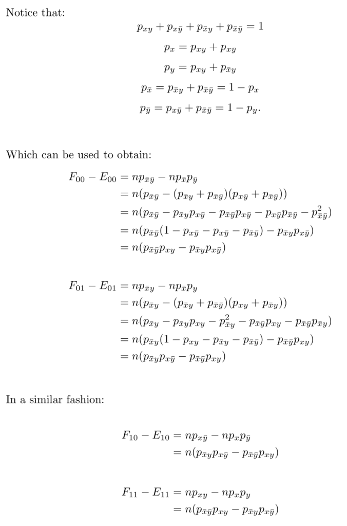
And that’s it! Now you may be wondering, what is the insight that this little exercise left me with? It’s actually very subtle, but also very interesting:

Generally speaking, we teach our Intro Stats students that a correlation of 0 does not imply independence, right? Easy example: Take , define and try to find the Pearson correlation between those two. Although they are perfectly dependent (Y is a function of X, after all) the non-monotonic relationship induced by the squaring (i.e., a parabola), “breaks” the linearity that the Pearson correlation is capturing. There is an important exception to this, though: jointly normally-distributed random variables (i.e., a multivariate normal distribution). In this case, a correlation of 0 does imply independence among the components of the multivariate structure. HOWEVER, notice the proof above. The (non-parametric) measure of dependency captured by the statistic, can also be expressed in terms of a correlation coefficient: the coefficient. Which means that for bivariate, Bernoulli distributed random variables, a correlation of 0 necessarily implies independence between the binary variables.

So now the list grows. Joint distributions for which a Pearson correlation of 0 implies independence:

(*) The multivariate normal

(*) The bivariate Bernoulli (but only the bivariate case).

This entry offers a quick tutorial on how to use the accompanying code to my article Theoretical considerations when simulating data from the g-and-h family of distributions, co-authored with Dr. Edward Kroc

The code works in two steps that need to be run independently to economize time and make the process of of simulation more efficient. It implements the theory outlined in Kowalchuk & Headrick (2010) with additional modifications described in my article. The most important one being the use of homotopy continuation to estimate the multiple roots of the system of transcendental equations that describe the skewness and (excess) kurtosis of the g-and-h family of distributions. Let us proceed with an example.

Let’s pretend for a moment that you would like to simulate a tri-variate g-and-h random variable. You would like each 1-D marginal distribution to have a skewness of 2 and an excess kurtosis of 7. You would also like them to be equally correlated at

The first step is finding the values for the (g,h) parameters that would give you the skewness and excess kurtosis of your choice. To do that, you would run the gh_roots() function which takes as an input (1) a vector of skewness parameters (one for each 1-D marginal); (2) a vector of excess kurtosis parameters; (3) the number of interval divisions in [0,1] to execute the homotopy continuation (uses the letter ‘m’ and the default set at 10); and (4) the number of attempted solutions to get (default set at 100). I have found that these numbers work well, but if you would like to find more than one pair of (g,h) parameters for the same values of skewness and excess kurtosis, you need to increase both the m number and the number of random attempts. Yes, the more you increase these numbers, the longer it takes R to find all solutions. Depending on the values of skewness and kurtosis, this could run for several minutes (like 5min-10min) to a full hour. Or more. This example is easy, so it’ll only take a few minutes. So one would do something like:

gh_roots(skew=2, kurt=7, m=10, tries=100)
[1] "3 solution(s) found for a skewness of 2 and a kurtosis of 7"
$g
[,1] [,2] [,3]

Var1 .4613686 .3998958 6.749384

$h

[,1] [,2] [,3]

Var1 .02466843 .0464031 -78.60594

You’ll get some other numbers that don’t really matter as well as a nice arrangement at the end that pairs each g parameter with its corresponding h parameter. For my purposes, let’s say I want to use the first pair so that g=.4613686 and h=.02466843

Now that you’ve chosen the parameters that will give you the population skewness and excess kurtosis of your choice, the next step is figuring out what the intermediate correlation matrix should be. If the concept of the ‘intermediate correlation matrix’ is new to you, please read this entry blog of mine.

To actually simulate the trivariate g-and-h distribution, you’ll now use the multgh() function. This one takes as arguments: (1) Sample size N (default set at 30); (2) vector of g parameters; (3) vector of h parameters; and (4) a population correlation matrix Sigma of your choice. Remember, Sigma needs to be the correlation matrix that *you*, the user, want as a population parameter. mutlgh() will use the theoretical framework described in Kowalchuk & Headrick (2010) , to calculate the intermediate correlation and actually simulate the data with g-and-h distributed marginals.

So, for our example above we can do:

set.seed(123)

n <- 10000

g1 <- c(.4613686, .4613686, .4613686)

h1 <- c(.02466843, .02466843, .02466843)

Sigm <- matrix(c(1, .5, .5, .5, 1, .5, .5, .5, 1),3, 3)

dat <- multgh(N=n, g=g1, h=h1, Sigma=Sigm)$data

And if you do:

> cor(dat)
          [,1]      [,2]      [,3]
[1,] 1.0000000 0.5039843 0.5211398
[2,] 0.5039843 1.0000000 0.4989272
[3,] 0.5211398 0.4989272 1.0000000

And use the describe() function in the psych package you can see that:

> describe(dat)
   vars     n mean   sd median trimmed  mad   min   max range skew kurtosis   
X1    1 10000 0.25 1.23  -0.01     0.1 0.97 -2.16 12.75 14.91 1.85     7.01 
X2    2 10000 0.24 1.24  -0.01     0.1 0.99 -2.03 16.85 18.88 1.93     9.15 
X3    3 10000 0.25 1.24  -0.02     0.1 0.98 -2.34 12.68 15.03 1.73     6.18 

So the skewness and (excess) kurtosis match the intended population values. If you’re new to the world of simulation, higher-order moments (skewness, kurtosis and whatnot) require REALLY large samples to be estimated consistently. We’re talking about 100s of thousands or millions. The larger they are, the larger the sample needed. So, for my purposes, I know this works well.

NOW THAT YOU’VE SPENT SOME TIME LEARNING HOW TO USE THIS METHOD, PLEASE REFER TO MY GITHUB TO GET THE FUNCTIONS.