I… am a weird guy (but then again, that isn’t news, hehe). And weird people sometimes have weird pet-peeves. Melted cheese on Italian food and hamburgers? Great! I’ll take two. Melted cheese anywhere else? Blasphemy! That obviously extends to Statistics. And one of my weird pet peeves (which was actually strong enough to prompt me to write it as a chapter for my dissertation and a subsequent published article) is when people conflate the Pearson and the Spearman correlation.
The theory of what I am going to talk about is developed in said article but when I was cleaning more of my computer files I found an interesting example that didn’t make it there. Here’s the gist of it:
I really don’t get why people say that the Spearman correlation is the ‘robust’ version or alternative to the Pearson correlation. Heck, even if you simply google the words Spearman correlation the second top hit reads
Spearman’s rank-order correlation is the nonparametric version of the Pearson product-moment correlation
When I read that, my mathematical mind immediately goes to “if this is the non-parametric version of the Pearson correlation, that means it also estimates the same population parameter”. And honest to G-d (don’t quote me on that one, though. But I just *know* it’s true) I feel like the VAST MAJORITY of people think exactly that about the Spearman correlation. And I wouldn’t blame them either… you can’t open an intro textbook for social scientists that doesn’t have some dubious version of the previous statement. “Well” – the reader might think- “if that is not true then why aren’t more people saying it?” The answer is that, for better or worse, this is one of those questions that’s very simple but the answer is mathematically complicated. But here’s the gist of it (again, for those who like theory like I do, read the article).
The Spearman rank correlation is defined, in the population, like this:
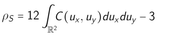
where the 


That relates the Pearson correlation 
I don’t remember why but I didn’t include this example in the article, but it is a very efficient one. It shows a case where the Spearman correlation is close to 1 but the Pearson correlation is close to 0 (obviously within sampling error).
Define 


N <- 1000000

Z <- rnorm(N, mean=0, sd=0.1)

X <- Z^201

Y <- exp(Z)
> cor(X,Y, method="pearson")

[1] 0.004009381
> cor(X,Y, method="spearman")

[1] 0.9963492
The trick for this example is to notice that the rate of change of 

In any case, the point being that even without being necessarily too formal, it’s not overly difficult to see that the Spearman correlation is its own statistic and estimates its own population parameter that may or may not have anything to do with the Pearson correlation, depending on the copula function describing the bivariate distribution.

You must be logged in to post a comment.