January | 2020 | psychometroscar

Us, academic reviewers, can be very finicky creatures (BTW don’t @me because deep down you know it is true. We’ve all been Reviewer 2 at least once in our careers 😜). Sometimes we miss the author(s)’ key points. Sometimes we review the paper that we think was written as opposed to the one that was actually written. And sometimes, we (serendipitously) offer the kind of keen insight into a problem that makes an author drop everything they’re doing and think “well, well, well… now THIS is interesting”. This story is about the latter type of review.

I will omit a lot of details here because our article has just been accepted (yay!) and we gotta respect the process. But the really cool stuff happened after the review so we’re all good. Anyway, here it goes: Reviews come in and they’re mostly short and positive. Change a few things here, add a few things there and we’re good to go. So everything is very hunky dory. As we’re working through them, this fine little piece catches my eyes (redacted):

It’s interesting to note that _________________ for uniform distributions (negative kurtosis), whereas _________________ concluded that _______________ is especially not robust to non-normal distributions with excess kurtosis (i.e., overestimated with negative kurtosis and underestimated with positive kurtosis), which does not seem to be in line with findings from this study. I wonder what the authors’ insight is on this particular aspect.

Now, it just so happens that _________________ was very thorough with their description of their simulation study and I could actually reproduce what they were doing. Also, as luck would have it, _________________ used a data-generating method that I am very, VERY familiar with. They used the 5th order power polynomial transformation which I myself used in the very first article I ever published. And here is the thing. If you compare the data _________________used as opposed to the one I used (uniform distributions) They appear to be very, very similar if you just look at the descriptives. Here’s the R output comparing the uniform distribution to the distribution used by _________________ (results are standardized to ease comparison):

vars n mean sd median trimmed mad min max range skew kurtosis se them 1000000 0 1 0 0 1.41 -2.34 2.34 4.68 0 -1.4 0 me 1000000 0 1 0 0 1.28 -1.73 1.73 3.46 0 -1.2 0

So… at least on paper these two things look the same. And I’d have a hard time believing that a -0.2 difference between (excess) kurtosis would result in all of this. Nevertheless, the advantage of working with the 5th order polynomial approach is that (whether you are interested in them or not), it allows the user control over the 5th and 6th central moments (so the next 2 moments after kurtosis). I would venture out a guess as to say you have probably never heard of those. Maybe you have never even seen how they look like. Luckily, with a little bit of algebra (and some help from Kendall & Stuart (1977) who defined the first six cumulants) it’s not too hard to show that the 5th and 6th (standardized) central moments are:

$\gamma_5=\frac{\int_{-\infty}^{\infty}(x-\mu)^5dF(x)}{[\int_{-\infty}^{\infty}(x-\mu)^2dF(x)]^{5/2}}-10\gamma_3$

$\gamma_6=\frac{\int_{-\infty}^{\infty}(x-\mu)^6dF(x)}{[\int_{-\infty}^{\infty}(x-\mu)^2dF(x)]^{3}}-15\gamma_4-10\gamma_3-15$

where $F(x)$ is the cumulative density function (CDF), $\gamma_3$ is the skewness and $\gamma_4$ is the excess kurtosis. Now I know that the distributions that _________________ used were symmetric along the mean so $\gamma_5=0$ because all the odd moments of a symmetric distribution are 0. And I know that $\gamma_6=22$ because if you know the coefficients used in the 5th order transformation, you can sort of “reverse-engineer” what the central moments of the distribution were. Which means all I had to do was figure out what $(\gamma_5, \gamma_6)$ are for the uniform distribution. Again, for the uniform distribution $\gamma_5=0$ by the same symmetry argument. So I just need to know that $\gamma_6$ is. Using the standard uniform CDF (so defined in the interval [0,1]) and the definition of central moments I need to solve for:

$\gamma_6=\frac{\int_{0}^{1}(x-1/2)^6dx}{[\int_{0}^{1}(x-1/2)^2dx]^{3}}-15(-6/5)-10(0)-15=\frac{48}{7} \approx 6.9$

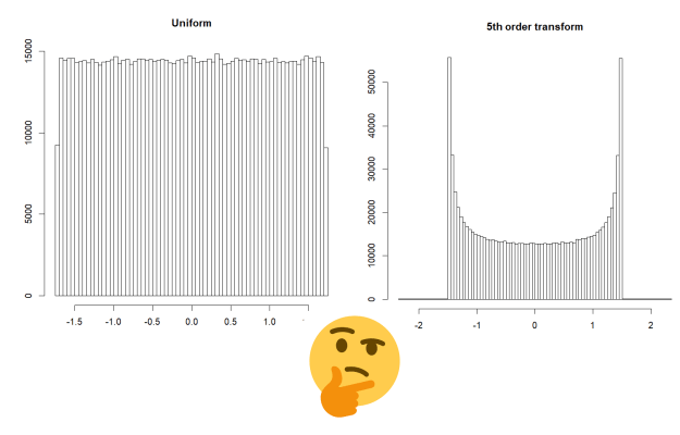
So… it seems like I can more or less match these two distributions all the way up to the 6th moment, which is where they become VERY different. Now, as expected, the big reveal is…. how do they look like when you graph them? Well, they look like this:

kurt_bimod

Yup, yup… there seems to be some bimodality going on here. It sort of looks like a beta distribution with equal parameters of 0.5, with the exception that the beta distribution is not defined outside the [0,1] range.

As usual, the next step is to figure out whether using one VS the other one could matter. I happen to be doing a little bit of research into tests for differences between correlations so I thought this would be a good opportunity to try this one out. I’m starting off with the easy-cheezy, t-test for two dependent correlations that Hotelling (1940) came up with. In any case, the t-statistic is expressed as follows:

$t=\frac{(r_{x_{1}y}-r_{x_{2}y})\sqrt{(n-3)(1+r_{x_{1}x_{2}})}}{det(\mathbf{R})}$

where $r_{x_{1}y}$ and $r_{x_{2}y}$ are the two correlations whose difference you are interested in, $r_{x_{1}x_{2}}$ is the correlation that induces the dependency and $det(\mathbf{R})$ is the determinant of the correlation matrix. So you have three variables at play here, $x_1, x_2$ and $y$ so the correlation matrix has dimensions $3 \times 3$ .

Alrighty, so here is the set-up for the small-scale simulation. I am gonna check the empirical Type I error rate of this t-test for the differences between correlations. I am setting up the 3 variables to be correlated equally with $\rho=0.5$ in the population. As simulation “conditions” I am using the two types of non-normalities discussed above: the uniform distribution VS the 5th-order-polynomial-transformed distribution. BTW, I am going to start calling them “Headrick distributions” in honour of Dr. Todd Headrick who laid the theoretical foundation for this area of research).

The uniform distribution part is easy because we can just use a Gaussian copula which ensures the distribution of the marginals is in fact the distribution that we intend (uniform). The 5th order polynomial part is a little bit more complicated. But since I figured out how to do this in R a while ago, then I know what should go in place of the intermediate correlation matrix (if this concept is new to you, please check out this blog of mine). In any case, simulation code:

set.seed(112) library(MASS)

nn<-100 #sample size reps<-1000 #replications h<-double(reps) #vector to store results c<-double(reps) #vector to store results

for(i in 1:reps){

##5th order polynomial transform

Z<-mvrnorm(nn, c(0,0,0), matrix(c(1,.60655,.60655,.60655,1,.60655,.60655,.60655,1),3,3)) z1<-Z[,1] z2<-Z[,2] z3<-Z[,3]

y1<-1.643377*z1-0.319988*z1^3+0.011344*z1^5 y2<-1.643377*z2-0.319988*z2^3+0.011344*z2^5 y3<-1.643377*z3-0.319988*z3^3+0.011344*z3^5
Y<-cbind(y1,y2,y3)

##############################################
##Gaussian copula

X <- mvrnorm(nn, c(0,0,0), matrix(c(1,.5189,.5189,.5189,1,.5189,.5189,.5189,1),3,3)) U <- pnorm(X)

q1<-qunif(U[,1] ,min=0, max=1) q2<-qunif(U[,2] ,min=0, max=1) q3<-qunif(U[,3] ,min=0, max=1)

Q<- cbind(q1,q2,q3)

###############################################

r12<-cor(y1,y2) r13<-cor(y1,y3) r23<-cor(y2,y3)

rq1q2 <- cor(q1, q2) rq1q3 <- cor(q1, q3) rq2q3 <- cor(q2, q3)

################################################ ##Test statistic from Hotelling (1940)

tt1<-(rq1q2-rq1q3)*sqrt(((nn-3)*(1+rq2q3)) / (2*det(cor(Q)))) c[i]<-2*pt(-abs(tt1),df=nn-3)

tt2<-(r12-r13)*sqrt(((nn-3)*(1+r12)) / (2*det(cor(Y)))) h[i]<-2*pt(-abs(tt2),df=nn-3)

} ############################################### #Empirical Type I error rates

>sum(h<.05)/reps
[1] 0.09
>sum(c<.05)/reps
[1] 0.056

Well, well, well… it appears that there *is* something interesting about the Headrick distribution that isn’t just there for the uniform. I mean, the uniform distribution is showing me a very good empirical Type I error rate. I’m sure a few more replications would get that rid of that additional .006 . But for the Headrick distribution the Type I error rate almost doubled. It does seem like whatever weirdness is going on in those tails may be playing a role on this… or maybe not? You see, I am beginning to wonder these days whether or not the definitions of moments beyond the variance are actually all that useful. I myself have a small collection of pictures of distributions that look somewhat (or VERY) different, yet have the same mean, variance, skewness and excess kurtosis. I use them in my intro classes to highlight to my students the importance of plotting your data.

Now, it could very well be the case that moments beyond the 4th only matter to differences of correlations and nothing else. Or maybe they do matter to other techniques. Which makes me wonder further… how far down the line of moments are we supposed to go before we can safely claim that X or Y statistical technique is robust? Sometimes I think we would be better off trying to make claims about families of probability distributions as opposed to distributions that exhibit certain values of certain moments. After all, Stoyanov’s famous book on counter examples in probability has a whole section of “moment problems” that highlights how one can build families of distributions with the same (finite) number of moments yet they are not the same type of distributions.

In any case, I guess the only sensible conclusion I can get from this is the good, ol’ “clearly, more research is needed” ¯\_(ツ)_/¯

psychometroscar

Monthly Archives: January 2020

Upper bounds on correlations and Cronbach’s alpha for discrete random variables

CLICK HERE FOR THE ACTUAL ARTICLE

YOU CAN CLICK HERE TO ACCESS THE APP

Is there life beyond the 4th (central) moment?