Here is a quick tutorial on how to use the Robbins-Monro method of stochastic root searching to estimate the intermediate correlation matrix that initializes the NORTA method. This method is described in the article Simultaneous estimation of the intermediate correlation matrix for arbitrary marginal densities co-authored with Dr. Bruno Zumbo and Dr. Edward Kroc. (It’s still in-press, so expect this entry to be updated once we can link to the actual article)

First, we need to decide what the final correlation matrix will be (the one we are interested in simulating from). In our article we simulated data from a 3-factor model with equal inter-factor correlations of 0.3, equal loadings of 0.7 and equal error variances of 0.51. The final correlation matrix is therefore:

L <- matrix(c(0.7, 0.7, 0.7,
              0.0, 0.0, 0.0,
              0.0, 0.0, 0.0,
              0.0, 0.0, 0.0,
              0.7, 0.7, 0.7, 
              0.0, 0.0, 0.0, 
              0.0, 0.0, 0.0,
              0.0, 0.0, 0.0, 
              0.7, 0.7, 0.7),9,3)

Phi <- matrix(c(1.0, 0.3, 0.3,
              0.3, 1.0, 0.3, 
              0.3, 0.3, 1.0),3,3)

Psi <- diag(9)

diag(Psi) <- 0.51

Sigm <- L%*%Phi%*%t(L) + Psi

Cx <-  Sigm

m <- dim(Cx)[1]

Next, one needs to decide on the types of marginal distributions and parameters one would want to simulate from. To highlight the flexibility of the method, a variety of marginal distributions (some discrete, some continuous) are used. The densities are specified as:

list_dist <- list(function(L) qchisq(L,df=1), 
                 function(L) qt(L,df=5), 
                 function(L) qbinom(L,5,0.5), 
                 function(L) qbeta(L, shape1=1, shape2=5), 
                 function(L) qpois(L, lambda=7), 
                 function(L) qgamma(L, shape=3, rate=5),
                 function(L) qnorm(L,mean=0, sd=1), 
                 function(L) qunif(L,min=0, max=1), 
                 function(L) qbinom(L,1,0.3))

M<- c(1, 
     0, 
     5*0.5, 
     1/(1+5), 
     7, 
     3/5,
     0, 
     0.5, 
     1*0.3)

S <- c(sqrt(2), 
      sqrt(5/(5-2)), 
      sqrt(5*0.5*0.5), 
      sqrt(5/((1+5)^2*(1+5+1))), 
      sqrt(7), 
      sqrt(3/5^2),
      sqrt(1), 
      sqrt(1/12), 
      sqrt(1*0.7*0.3))

MM <- M%*%t(M)
SS <- S%*%t(S)

The ‘M‘ and ‘S‘ variables are for ‘mean’ and ‘standard deviation’ respectively. Notice how the entries follow the same order as the distributions in the list_dist list. Also, keep an eye on the matrix approach to encode this information with ‘MM‘ and ‘SS‘. The function that estimates the intermediate correlation matrix needs these entries.

Once the final correlation matrix and the marginal densities are been decided on, we have all the elements we need to estimate the intermediate correlation matrix:

#Final correlation as starting point
C0 <- Cx

#Increasing iterations (iter) and tolerance (tol) increases the accuracy of 
#estimation, but it also increases computing time. 
iter<-500 
tol<-0.001

#Can only take values in (0,1). Values close to 1 increase the accuracy of 
#estimation, but it also increases computing time.  
alph<-0.75
a<-1

#Sample size to verify empirical approximation. We recommend to set it at 
#100,000
n<-100000

### Computation of Cz ###
##################################################################
L<-RM(C0,Cx,MM,SS,list_dist,a,iter,tol,n,alph)
Cz<-L[[1]]
Cx_est<-GN(Cz,Cx,MM,SS,list_dist,n)

And now that all the elements are in place, please find the link to the RM() function that implements the stochastic root searching.

PLEASE REFER TO MY GITHUB FOR THE FUNCTION

There’s no way around it: I’m a fan of procrastinating. But I try to procrastinate in ways that teach me something or that help me learn… which is why one of the things I like to do when procrastinating is figuring out algebraic relationships of things. Which brings us to this nice little result that taught me something a tad bit deeper than I expected. Let me begin.

A few months ago an interesting question was posed on Twitter inquiring about the relationship between the test of association for contingency tables and logistic regression. It was a very interesting thread, but within it there were a couple of tweets that captured my attention, which you can find here in case you’d like to know the context. I do reproduce them here just for the sake of keeping this blog entry self-contained:

Now, because I’m a huge stats nerd, I know that the test of association can be fit as a logistic regression model, and I also know that the coefficient (i.e., the Pearson correlation between two binary variables) follows the relationship when working with 2×2 tables. What I don’t know (and had actually never seen worked out) is why?

So the first thing I do is go to the Wikipedia entry for the coefficient. And there is a reference there. One of the classics of psychometrics, Guilford’s (1936) Psychometric Methods. I have it. I go and check it and on p.432 I see:

That’s it. No proof, no explanation. Just a throwaway statement that these things are equal without elaboration. Perhaps Lord & Novick’s (1968) Statistical Theories of Mental Test Scores can offer some guidance? I mean, that book has everything psychometrics in it. I go. I check. And I find this on p.336:

Again, no luck. But a clue has been offered: “It can be shown after tedious algebra (…)”. If you’ve read old math/stats books/articles/etc. (they don’t mince words when describing things), then you know the chances of finding out a formal proof of this are slim to none. This is one of those things that amounts to what I call a “bookkeeping proof”. The kind of proof that relies mostly on being careful with how things are defined, which subscripts should be used where, etc., but the technique is really just pushing around algebraic symbols. Which is perfect for me, because that’s what I like to do to procrastinate! So I decided that it would probably be a good idea to work this out and leave it available somewhere (like on this blog), to make sure people in the future don’t have to work through tedious algebra. So…here it is! And to put the cherry on top, it did help me realize something that I’d never seen before.

WordPress makes it difficult (at least for me) to include large chunks of LaTeX, so I’ll take the more humble approach of uploading the proof as pictures.

And that’s it! Now you may be wondering, what is the insight that this little exercise left me with? It’s actually very subtle, but also very interesting:

Generally speaking, we teach our Intro Stats students that a correlation of 0 does not imply independence, right? Easy example: Take , define and try to find the Pearson correlation between those two. Although they are perfectly dependent (Y is a function of X, after all) the non-monotonic relationship induced by the squaring (i.e., a parabola), “breaks” the linearity that the Pearson correlation is capturing. There is an important exception to this, though: jointly normally-distributed random variables (i.e., a multivariate normal distribution). In this case, a correlation of 0 does imply independence among the components of the multivariate structure. HOWEVER, notice the proof above. The (non-parametric) measure of dependency captured by the statistic, can also be expressed in terms of a correlation coefficient: the coefficient. Which means that for bivariate, Bernoulli distributed random variables, a correlation of 0 necessarily implies independence between the binary variables.

So now the list grows. Joint distributions for which a Pearson correlation of 0 implies independence:

(*) The multivariate normal

(*) The bivariate Bernoulli (but only the bivariate case).

This entry offers a quick tutorial on how to use the accompanying code to my article Theoretical considerations when simulating data from the g-and-h family of distributions, co-authored with Dr. Edward Kroc

The code works in two steps that need to be run independently to economize time and make the process of of simulation more efficient. It implements the theory outlined in Kowalchuk & Headrick (2010) with additional modifications described in my article. The most important one being the use of homotopy continuation to estimate the multiple roots of the system of transcendental equations that describe the skewness and (excess) kurtosis of the g-and-h family of distributions. Let us proceed with an example.

Let’s pretend for a moment that you would like to simulate a tri-variate g-and-h random variable. You would like each 1-D marginal distribution to have a skewness of 2 and an excess kurtosis of 7. You would also like them to be equally correlated at

The first step is finding the values for the (g,h) parameters that would give you the skewness and excess kurtosis of your choice. To do that, you would run the gh_roots() function which takes as an input (1) a vector of skewness parameters (one for each 1-D marginal); (2) a vector of excess kurtosis parameters; (3) the number of interval divisions in [0,1] to execute the homotopy continuation (uses the letter ‘m’ and the default set at 10); and (4) the number of attempted solutions to get (default set at 100). I have found that these numbers work well, but if you would like to find more than one pair of (g,h) parameters for the same values of skewness and excess kurtosis, you need to increase both the m number and the number of random attempts. Yes, the more you increase these numbers, the longer it takes R to find all solutions. Depending on the values of skewness and kurtosis, this could run for several minutes (like 5min-10min) to a full hour. Or more. This example is easy, so it’ll only take a few minutes. So one would do something like:

gh_roots(skew=2, kurt=7, m=10, tries=100)
[1] "3 solution(s) found for a skewness of 2 and a kurtosis of 7"
$g
[,1] [,2] [,3]

Var1 .4613686 .3998958 6.749384

$h

[,1] [,2] [,3]

Var1 .02466843 .0464031 -78.60594

You’ll get some other numbers that don’t really matter as well as a nice arrangement at the end that pairs each g parameter with its corresponding h parameter. For my purposes, let’s say I want to use the first pair so that g=.4613686 and h=.02466843

Now that you’ve chosen the parameters that will give you the population skewness and excess kurtosis of your choice, the next step is figuring out what the intermediate correlation matrix should be. If the concept of the ‘intermediate correlation matrix’ is new to you, please read this entry blog of mine.

To actually simulate the trivariate g-and-h distribution, you’ll now use the multgh() function. This one takes as arguments: (1) Sample size N (default set at 30); (2) vector of g parameters; (3) vector of h parameters; and (4) a population correlation matrix Sigma of your choice. Remember, Sigma needs to be the correlation matrix that *you*, the user, want as a population parameter. mutlgh() will use the theoretical framework described in Kowalchuk & Headrick (2010) , to calculate the intermediate correlation and actually simulate the data with g-and-h distributed marginals.

So, for our example above we can do:

set.seed(123)

n <- 10000

g1 <- c(.4613686, .4613686, .4613686)

h1 <- c(.02466843, .02466843, .02466843)

Sigm <- matrix(c(1, .5, .5, .5, 1, .5, .5, .5, 1),3, 3)

dat <- multgh(N=n, g=g1, h=h1, Sigma=Sigm)$data

And if you do:

> cor(dat)
          [,1]      [,2]      [,3]
[1,] 1.0000000 0.5039843 0.5211398
[2,] 0.5039843 1.0000000 0.4989272
[3,] 0.5211398 0.4989272 1.0000000

And use the describe() function in the psych package you can see that:

> describe(dat)
   vars     n mean   sd median trimmed  mad   min   max range skew kurtosis   
X1    1 10000 0.25 1.23  -0.01     0.1 0.97 -2.16 12.75 14.91 1.85     7.01 
X2    2 10000 0.24 1.24  -0.01     0.1 0.99 -2.03 16.85 18.88 1.93     9.15 
X3    3 10000 0.25 1.24  -0.02     0.1 0.98 -2.34 12.68 15.03 1.73     6.18 

So the skewness and (excess) kurtosis match the intended population values. If you’re new to the world of simulation, higher-order moments (skewness, kurtosis and whatnot) require REALLY large samples to be estimated consistently. We’re talking about 100s of thousands or millions. The larger they are, the larger the sample needed. So, for my purposes, I know this works well.

NOW THAT YOU’VE SPENT SOME TIME LEARNING HOW TO USE THIS METHOD, PLEASE REFER TO MY GITHUB TO GET THE FUNCTIONS.

CLICK HERE FOR THE ACTUAL ARTICLE

This is a small tutorial on how to either use the R code (if you are an R user) or the web application (if you prefer a user-friendly GUI) that will calculate the upper bound on (positive) correlations between random variables with an arbitrary number of categories.

The first thing to know is that your categories should start at 0 (not 1). If you are using the R code, please make sure your categories start there. If you are using the GUI, it will check (variable by variable) whether or not the categories start at 0 and will make the necessary adjustments for you.

The overall interface is very simple:

The first step will be to upload your data where it says “Browse”. Notice that:

(1) This app ONLY takes .csv files. If you are an SPSS user and are unfamiliar with how to save your SPSS (extension .sav) data as a .csv file, here is an easy explanation. Trust me, it’s A LOT easier than you think.

(2) It will use ALL the variables in your data file. If you have other variables or covariates which you are not interested in correlating, you have to remove them before uploading the data.

(3) It doesn’t handle missing data. You need to provide a .csv file with no missing elements so you need to ‘pre-process’ it before you upload it.

And…. that’s pretty much it. Once you’ve pre-processed the data and uploaded the file just click “Run” and it should give you something that looks like this:

The interpretation is very simple. It uses the number of categories and the probabilities of endorsing each category to calculate the maximum possible correlations that you could have observed. Then it uses this convenient formula that operates exclusively on the correlation (or the covariance) matrix to calculate Cronbach’s alpha. Keep in mind that this would be the standardized Cronbach’s alpha (as opposed to the raw one). But you can always use it as a point of reference. Or work backwards from the maximum possible correlation matrix and “unstandardize” it to obtain the maximum possible covariance matrix.

If you have many variables, the correlation matrix won’t be displayed. But you can download it as a .csv file for inspection or click on ‘copy’ to copy-paste it in Microsoft Words or some text editor of your choice. Cronbach’s alpha is always calculated.

And… that is pretty much it.

YOU CAN CLICK HERE TO ACCESS THE APP

And if you are an R user and feel more at home with code, HERE IS THE CODE THAT RUNS THE ANALYSIS.

Us, academic reviewers, can be very finicky creatures (BTW don’t @me because deep down you know it is true. We’ve all been Reviewer 2 at least once in our careers 😜). Sometimes we miss the author(s)’ key points. Sometimes we review the paper that we think was written as opposed to the one that was actually written. And sometimes, we (serendipitously) offer the kind of keen insight into a problem that makes an author drop everything they’re doing and think “well, well, well… now THIS is interesting”.  This story is about the latter type of review.

I will omit a lot of details here because our article has just been accepted (yay!) and we gotta respect the process. But the really cool stuff happened after the review so we’re all good. Anyway, here it goes: Reviews come in and they’re mostly short and positive. Change a few things here, add a few things there and we’re good to go. So everything is very hunky dory. As we’re working through them, this fine little piece catches my eyes (redacted):

It’s interesting to note that _________________  for uniform distributions (negative kurtosis), whereas _________________ concluded that _______________ is especially not robust to non-normal distributions with excess kurtosis (i.e., overestimated with negative kurtosis and underestimated with positive kurtosis), which does not seem to be in line with findings from this study. I wonder what the authors’ insight is on this particular aspect.

Now, it just so happens that _________________ was very thorough with their description of their simulation study and I could actually reproduce what they were doing. Also, as luck would have it, _________________ used a data-generating method that I am very, VERY familiar with. They used the 5th order power polynomial transformation which I myself used in the very first article I ever published. And here is the thing. If you compare the data _________________used as opposed to the one I used (uniform distributions) They appear to be very, very similar if you just look at the descriptives. Here’s the R output comparing the uniform distribution to the distribution used by _________________ (results are standardized to ease comparison):

vars     n mean sd median trimmed   mad    min  max range skew kurtosis  se
them 1000000   0   1     0        0 1.41 -2.34 2.34  4.68     0    -1.4   0
me   1000000   0   1     0        0 1.28 -1.73 1.73  3.46     0    -1.2   0

So… at least on paper these two things look the same. And I’d have a hard time believing that a -0.2 difference between (excess) kurtosis would result in all of this. Nevertheless, the advantage of working with the 5th order polynomial approach is that (whether you are interested in them or not), it allows the user control over the 5th and 6th central moments (so the next 2 moments after kurtosis).  I would venture out a guess as to say you have probably never heard of those. Maybe you have never even seen how they look like. Luckily, with a little bit of algebra (and some help from Kendall & Stuart (1977) who defined the first six cumulants) it’s not too hard to show that the 5th and 6th (standardized) central moments are:

where is the cumulative density function (CDF), is the skewness and is the excess kurtosis. Now I know that the distributions that _________________ used were symmetric along the mean so because all the odd moments of a symmetric distribution are 0. And I know that because if you know the coefficients used in the 5th order transformation, you can sort of  “reverse-engineer” what the central moments of the distribution were. Which means all I had to do was figure out what are for the uniform distribution. Again, for the uniform distribution by the same symmetry argument. So I just need to know that is. Using the standard uniform CDF (so defined in the interval [0,1]) and the definition of central moments I need to solve for:

So… it seems like I can more or less match these two distributions all the way up to the 6th moment, which is where they become VERY different. Now, as expected, the big reveal is…. how do they look like when you graph them? Well, they look like this:

Yup, yup… there seems to be some bimodality going on here. It sort of looks like a beta distribution with equal parameters of 0.5, with the exception that the beta distribution is not defined outside the [0,1] range.

As usual, the next step is to figure out whether using one VS the other one could matter. I happen to be doing a little bit of research into tests for differences between correlations so I thought this would be a good opportunity to try this one out. I’m starting off with the easy-cheezy, t-test for two dependent correlations that Hotelling (1940) came up with. In any case, the t-statistic is expressed as follows:

where and are the two correlations whose difference you are interested in, is the correlation that induces the dependency and is the determinant of the correlation matrix. So you have three variables at play here, and so the correlation matrix has dimensions .

Alrighty, so here is the set-up for the small-scale simulation. I am gonna check the empirical Type I error rate of this t-test for the differences between correlations. I am setting up the 3 variables to be correlated equally with in the population. As simulation “conditions” I am using the two types of non-normalities discussed above: the uniform distribution VS the 5th-order-polynomial-transformed distribution. BTW, I am going to start calling them “Headrick distributions” in honour of Dr. Todd Headrick who laid the theoretical foundation for this area of research).

The uniform distribution part is easy because we can just use a Gaussian copula which ensures the distribution of the marginals is in fact the distribution that we intend (uniform).  The 5th order polynomial part is a little bit more complicated. But since I figured out how to do this in R a while ago, then I know what should go in place of the intermediate correlation matrix (if this concept is new to you, please check out this blog of mine). In any case, simulation code:

set.seed(112)
library(MASS)

nn<-100 #sample size
reps<-1000 #replications
h<-double(reps) #vector to store results
c<-double(reps) #vector to store results

for(i in 1:reps){

##5th order polynomial transform

Z<-mvrnorm(nn, c(0,0,0), matrix(c(1,.60655,.60655,.60655,1,.60655,.60655,.60655,1),3,3))
z1<-Z[,1]
z2<-Z[,2]
z3<-Z[,3]

y1<-1.643377*z1-0.319988*z1^3+0.011344*z1^5
y2<-1.643377*z2-0.319988*z2^3+0.011344*z2^5
y3<-1.643377*z3-0.319988*z3^3+0.011344*z3^5

Y<-cbind(y1,y2,y3)

##############################################

##Gaussian copula

X <- mvrnorm(nn, c(0,0,0), matrix(c(1,.5189,.5189,.5189,1,.5189,.5189,.5189,1),3,3))
U <- pnorm(X)

q1<-qunif(U[,1] ,min=0, max=1)
q2<-qunif(U[,2] ,min=0, max=1)
q3<-qunif(U[,3] ,min=0, max=1)

Q<- cbind(q1,q2,q3)

###############################################

r12<-cor(y1,y2)
r13<-cor(y1,y3)
r23<-cor(y2,y3)

rq1q2 <- cor(q1, q2)
rq1q3 <- cor(q1, q3)
rq2q3 <- cor(q2, q3)

################################################
##Test statistic from Hotelling (1940)

tt1<-(rq1q2-rq1q3)*sqrt(((nn-3)*(1+rq2q3)) / (2*det(cor(Q))))
c[i]<-2*pt(-abs(tt1),df=nn-3)

tt2<-(r12-r13)*sqrt(((nn-3)*(1+r12)) / (2*det(cor(Y))))
h[i]<-2*pt(-abs(tt2),df=nn-3)

}
###############################################
#Empirical Type I error rates

>sum(h<.05)/reps
[1] 0.09
>sum(c<.05)/reps
[1] 0.056

Well, well, well… it appears that there *is* something interesting about the Headrick distribution that isn’t just there for the uniform. I mean, the uniform distribution is showing me a very good empirical Type I error rate. I’m sure a few more replications would get that rid of that additional .006 . But for the Headrick distribution the Type I error rate almost doubled. It does seem like whatever weirdness is going on in those tails may be playing a role on this… or maybe not? You see, I am beginning to wonder these days whether or not the definitions of moments beyond the variance are actually all that useful. I myself have a small collection of pictures of distributions that look somewhat (or VERY) different, yet have the same mean, variance, skewness and excess kurtosis. I use them in my intro classes to highlight to my students the importance of plotting your data.

Now, it could very well be the case that moments beyond the 4th only matter to differences of correlations and nothing else. Or maybe they do matter to other techniques. Which makes me wonder further… how far down the line of moments are we supposed to go before we can safely claim that X or Y statistical technique is robust? Sometimes I think we would be better off trying to make claims about families of probability distributions as opposed to distributions that exhibit certain values of certain moments. After all, Stoyanov’s famous book on counter examples in probability has a whole section of  “moment problems” that highlights how one can build families of distributions with the same (finite) number of moments yet they are not the same type of distributions.

In any case, I guess the only sensible conclusion I can get from this is the good, ol’ “clearly, more research is needed” ¯\_(ツ)_/¯

This came out of an email exchange that I had with my dear friend Ben Shear and I eventually realized it could benefit more people. If you have two log-normal random variables how can you correlate them the right way? When I say the right way I mean that you both get the population correlation that you want and the 1-dimensional marginals that you want.

Naive approach #1 (Wrong): Correlate first, transform later

This one is a popular one:

library(MASS)
mult_norm<- mvrnorm(1000, c(0,0), matrix(c(1,.5,.5,1),2,2))
log_norm<- exp(mult_norm)

This one gets you the right marginals (they are, indeed, log-normal). But the wrong correlation matrix as you can see:

cor(mult_norm)
[,1]      [,2]
[1,] 1.0000000 0.4967083
[2,] 0.4967083 1.0000000


> cor(log_norm)
[,1]      [,2]
[1,] 1.0000000 0.4419539
[2,] 0.4419539 1.0000000

The resulting correlation matrix is biased downwards. So that won’t do.

Naive approach #2 (Wrong as well): Transform first, correlate later

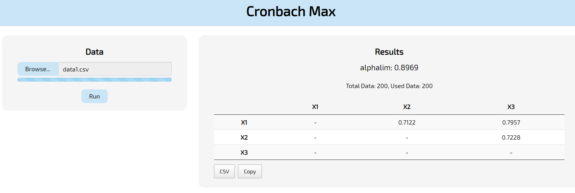
This one is also very appealing because of its simplicity and because it relies on the construction of a bivariate normal distribution. Like, if are each independent and identically distributed define . Then are bivariate normally distributed with and population correlation coefficient .

What would happen then if we did and did ?

In this case, would still be log-normal and . But would NOT be log-normally distributed. The Dufresne (2009) paper is the standard reference for this, but there have been some interesting developments, like this approximation using the log-skew-normal distribution. In any case, the distribution of isn’t known.

A third (correct) way

This is essentially a re-hash of Appendix A in Astivia & Zumbo (2017) where it’s not too difficult to show that if are standard bivariate normal with correlation coefficient then the correlation between is:

So what we can do is solve for above and find that:

And what we do is that we go back to Naive Approach #1 and plug **that** as the initial correlation coefficient so that, through the process of exponentiation, we get back the value for that we want our log-normal marginal distributions to have in the population.

Small simulation check:

library(MASS)

###I want a population correlation between
###the log-normals of 0.5 so:
rr<-double(1000)

for(i in 1:1000){
mult_norm<-mvrnorm(1000, c(0,0), matrix(c(1,log(.5*(exp(1)-1)+1),log(.5*(exp(1)-1)+1),1),2,2))

log_norm<-exp(mult_norm)

rr[i]<-cor(log_norm)[1,2]
}
mean(rr)
>0.5019529

And the joint distribution would look like this:

We usually call the correlation that we need to set for the initial bivariate normal the “intermediate correlation” and it gives us some interesting insights into how the correlation coefficient behaves when the marginals are not normal.

For example here if I wanted to give my log-normals a correlation I’d do:

log(-.5*(exp(1)-1)+1)
[1] -1.959995

And find out that I can’t. Two log-normal random variables generated from a standard bivariate normal distribution CANNOT be correlated at -0.5. The maximum possible negative correlation is actually .

While I am preparing for a more “in-depth” treatment of this Twitter thread that sparked some interest (thank my lucky stars!) , I ran into a couple of curious distributions that I think highlight an important lesson: not EVERYTHING needs a copula 😉 Sure, they’re flexible and powerful modelling approaches. But at the end of the day there are other methods to create multivariate, non-normal distributions. And many of them have very elegant theoretical properties that allow us to expand our the intuitions about these distributions from the univariate to the multivariate setting.

So here I present two distributions which can be generalized from their univariate to a multivariate definition without invoking a copula.

Multivariate Poisson Distribution

The Poisson distribution is closed under convolutions. For purposes of this post, that means that if and are independent, Poisson-distributed (with parameters respectively) then is also Poisson-distributed, (with parameter… Yup! You got it! ).

So let’s start easy, the bivariate case. To construct a bivariate Poisson random vector we can use the following stochastic representation:

Where are independent Poisson random variables with parameters respectively. Since Poisson distributions are closed under convolutions, and are Poisson distributed with variance  respectively, and covariance . Notice that this construction implies the restriction .

Using the above property we can derive the joint probability function of . Consider fixed values Since can take any values between 0 and and are mutually independent then we can use this property to define the joint probability function as:

where are the probability functions of respectively. By making the proper substitutions in the and some collecting of terms we have:

From this process I could expand it to, say, a trivariate Poisson random variable by expressing the 3-D vector as:

Where all the X’s are themselves independent, Poisson distributed and the terms with double (and triple) subscript would control the level of covariance among the Poisson marginal distributions.  If you repeat this iteratively adding more and more terms to the summation then you can increase the dimensions of the multivariate Poisson distribution.

Multivariate Exponential Distribution

The univariate exponential distribution is also (sort of) closed under convolution. But, in this very specific case, it’s closed under weighted minima convolution. For this post, that means that if are independent, exponential random variables, then is also exponentially-distributed for .

We can start very similarly as with the previous case by defining how the bivariate distribution would look like. Here we start with:

where are independent, exponentially-distributed random variables with parameters (I SWEAR to God the standard mathematical notation for the parameter of both the exponential and the Poisson distribution is . Of course would be chosen as the minima of their respective sequences of exponential random variables. Because of this are also exponentially-distributed with parameters respectively. Since are independent, then we have:

And the joint cumulative density function of the bivariate vector would then be:

Moral of the story

If you know me, you’ll know that I tend to be overly critical of the things I like the most, which is a habit that doesn’t always makes me a lot of friends, heh. Because I like copula modelling and I like the idea of non-normal, multivariate structures, I also like to see and understand the cases where defining multivariate structures that do not need a copula may give us insights. For the particular two cases above, I am exploiting the fact that sums of these types of random variables also result in the same type of random variable (i.e., closed under convolution) which, for better or worse, is a very useful property that not many univariate probability distributions have. Nevertheless, when they *do* have it, it is perhaps wise to use them because, at the end of the day, using copulas to either simulate or model multivariate data does not imply the copula distribution *becomes* the “multivariate” version of that distribution. A Gaussian copula with gamma-distributed marginals is not a “multivariate gamma distribution”. It is… well… a Gaussian copula with gamma distributed marginals. If you change the copula function for something else (say an Archimidean copula) the multivariate properties change as well. Which brings us to a very sobering realization: with the exception of some very select types of multivariate distributions (usually those closed under convolution) we don’t always have well-defined extensions of multivariate distributions. For example, there are more than 10 different ways to define distributions that would satisfy what one would call a “multivariate t distribution”. Whichever characterization one chooses is usually contingent on the intended use for it. I guess this helps highlight one of the oldest pieces of advice I ever received: You know you have become a good methodologist when you realize the only correct answer to every data analysis question is simply “it depends”. 

This app will perform computer simulations to estimate the power of the t-tests within a multiple regression context under the assumption that the predictors and the criterion variable are continuous and either normally or non-normally distributed. If you would like to see why I think this is important to keep in mind, please read this blog post.

When you first click on the app it looks like this:

What *you*, the user, needs to provide it with is the following:

The number of predictors. It can handle anything from 3 to 6 predictors. When you have more than that the overall aesthetics of the app is simply too crowded.  The default is 3 predictors.

The regression coefficients (i.e, the standardized effect sizes) that hold in the population. The default is 0.3. The app names them “x1, x2, x3,…x6”

The skewness and excess kurtosis of the data for each predictor AND for the dependent variable (the app calls it “y”). Please keep on reading to see how you should choose those. The defaults at this point are skewness of 2 and an excess kurtosis of 7.

The pairwise correlations among the predictors. I think this is quite important because the correlation among the predictors plays a role in calculating the standard error of the regression coefficients. So you can either be VERY optimistic and place those at 0 (predictors are perfectly orthogonal with one another) OR you can be very pessimistic and give them a high correlation (multicollinearity). The default inter-predictor correlation is 0.5.

The sample size. The default is 200.

The number of replications for the simulation. The default is 100.

Now, what’s the deal with the skewness and excess kurtosis? A lot of people do not know this but you cannot go around choosing values of skewness and excess kurtosis all willy-nilly. There is a quadratic relationship between the possible values of skewness and excess kurtosis that specifies they MUST be chosen according to the inequality kurtosis >skewness^2-2 . If you don’t do this, it will spit out an error. Now, I am **not** a super fan of the algorithm needed to generate data with those population-specified values of skewness and excess kurtosis. For many AND even more reasons. HOWEVER, I needed to choose something that was both sufficiently straight-forward to implement and not very computationally-intensive, so the 3rd order polynomial approach will have to do.

Now, the exact boundaries of what this method can calculate are actually smaller than the theoretical parabola. However, for practical purposes, as long as you choose values of kurtosis which are sufficiently far apart from the square of the skewness, you should be fine. So, a combo like skewness=3, kurtosis=7 would give it trouble. But something like skewness=3, kurtosis=15 would be perfectly fine.

A hypothetical run would look like this:

So the output under Results is the empirical, simulated power for each regression coefficient at the sample size selected. In this case, they gravitate around 60%.

Oh! And if for whatever reason you would like to have all your predictors be normal, you can set the values of skewness and kurtosis to 0. In fact, in that situation you would end up working with a multivariate normal distribution.

YOU CAN CLICK HERE TO ACCESS THE APP

This app will perform computer simulations to estimate the power of the t-test for the Pearson bivariate correlation under the assumption that the data are continuous and either bivariate normally distributed or non-normally distributed. To see why this is important, please check out this blog post.

It is very straightforward to use. When you click on the app, it will look like this:

What *you*, the user, needs to provide it with is the following:

The population correlation (i.e., the effect size) for which you would like to obtain power. The default is 0.3

The type of distributions you would like to correlate together. Right now it can handle the chi-square distribution (where skewness is controlled through the degrees of freedom), the uniform distribution (to have a symmetric distribution with negative kurtosis) and the binomial distribution where one can control the number of response categories (size) and the probability parameter. This will soon be replaced by a multinomial distribution so that the probability of every marginal response option can be specified.

The sample size. The default is 20

The number of replications for the simulation. The default is 100.

Now, what is the app actually doing? It runs R underneath and it is going to give you the estimated power of the t-test under both conditions. The first one is calculated under the assumption that your data are bivariate normally distributed. This is just a direct use of the pwr.r.test function of the pwr R package. Should give you answers very close or exactly the same as G*Power. I chose to use it for sake of comparison.

What comes out is something that looks like this:

So, on top, you’re going to get the power as if you were using G*Power (or the pwr R package) which is exact and needs no simulation because we have closed-form expressions for it. On the bottom you are going to get the approximated power using simulations. Remember, when working with non-normal data you can’t always expect power to be lower, as in this case. Sometimes it may be higher and sometimes it won’t change much. Yes, at some point (if your sample size is large enough) the distribution of your data will matter very little. But, in the meantime, at least you can use this one to guide you!

Finally, here’s the link for the shiny web app:

YOU CAN CLICK HERE TO ACCESS THE APP

So… here’s a trick I use sometimes that I’ve never seen anywhere else and it may be helpful to some people.

If you work with latent variable models, Factor Analysis, Structural Equation Modelling, Item Response Theory, etc. there’s a good chance that you have either encountered or have seen some version of a warning about a covariance matrix being “non positive definite”. This is an important warning because the software is telling you that your covariance matrix is not a valid covariance matrix and, therefore, your analysis is suspect. Usually, within the world of latent variables we call these types of warnings Heywood cases .

Now, most Heywood cases are very easy to spot because they pertain to one of two broad classes: negative variances or correlations greater than 1. When you inspect your matrix models and see either of those two cases, you know exactly which variable is giving you trouble. Thing is (as I found out a few years ago), there are other types of Heywood cases that are a lot more difficult to diagnose. Consider the following matrix that I once got helping a student with his analysis:


............space    lstnng    actvts    prntst    persnl    intrct    prgrmm
space       1.000
lstnng      0.599    1.000
actvts      0.706    0.646     1.000
prntst      0.702    0.459     0.653      1.000
persnl      0.591    0.582     0.844      0.776     1.00
intrct      0.627    0.964     0.501      0.325     0.639    1.000
prgrmm      0.493    0.602     0.981      0.687     0.944    0.642      1.000


This is the model-implied correlation matrix I obtained through the analysis which gave a Heywood case warning. The student was a bit puzzled because, although we had reviewed this type of situations in class, we had only mentioned the case of negative variances or correlations greater than one. Here he neither had a negative variance nor a correlation greater than one… but he still got a warning for non-positive definiteness.

My first reaction was, obviously, to check the eigenvalues of the matrix and, lo and behold, there it was:
[1] 5.01377877 1.00744933 0.62602056 0.30393170 0.16671742 0.01317704 -0.13107483

So… yeah. This was, indeed, an invalid correlation/covariance matrix and we needed to further diagnose where the problem was coming from… but how? Enter our good friend, linear algebra.

If you have ever taken a class in linear algebra beyond what’s required in a traditional methodology/statistics course sequence for social sciences, you may have encountered something called the minor of a matrix. Minors are important because they’re used to calculate the determinant of a matrix. They’re also important for cases like this one because they break down the structure of a matrix into simpler components that can be analyzed. Way in the back of my mind I remembered from my undergraduate years that positive-definite matrices had something special about their minors. So when I came home I went through my old, OLD notes and found this beautiful theorem known as Sylvester’s criterion:

A Hermitian matrix is positive-definite if and only if  all of the leading principal minors have positive determinant.

All covariance matrices are Hermitian (the subject for another blogpost) so we’re only left to wonder what is a principal minor. Well, if you imagine starting at the [1,1] coordinate of a matrix (so really the upper-left entry) and going downwards diagonally expanding one row and column at a time you’d end up with the principal minors. A picture makes a lot more sense for this:

So… yeah. The red square (so the q11 entry) is the first principal minor. The blue square (a 2 x 2 matrix) is the 2nd principal minor, the yellow square (a 3 x 3 matrix) is the 3rd principal minor and on it goes until you get the full n x n matrix. For the matrix Q to be positive-definite, all the n-1 principal minors need to have positive determinant. So if you want to “diagnose” your matrix for positive definiteness, all you need to do is start from the upper-left corner and check the determinants consecutively until you found one that is less than 0. Let’s start from the previous example. Notice that I’m calling the matrix ‘Q’:
1
> det(Q[1:2,1:2])
[1] 0.641199
> det(Q[1:3,1:3])
[1] 0.2933427
> det(Q[1:4,1:4])
[1] 0.01973229
> det(Q[1:5,1:5])
[1] 0.003930676
> det(Q[1:6,1:6])
[1] -0.003353769


The first [1,1] corner is a given (it’s a correlation matrix so it’s 1 and it’s positive). Then we move downwards the 2×2 matrix, the 3×3 matrix… all the way to the 5×5 matrix. By then the determinant of Q is very small so I suspected that whatever the issue might be, it had to do with the relationship of the variables  “persnl”,  “intrct” or “prgrmm”. The final determinant pointed towards the culprit. Whatever problem this matrix exhibited, it had to do with the relationship between “intrct” and”prgrmm”.

Once I pointed out to the student that I suspected the problem was coming from either one of these two variables, a careful examination revealed the cause: The “intrct” item was a reverse-coded item but, for some reason, several of the participants respondents were not reverse-coded. So you had a good chunk of the responses to this item pointing to one direction and a smaller (albeit still large) number pointing to the other direction. The moment this item was full reverse-coded the non-positive definite issue disappeared.

I guess there are two lessons to this story: (1) Rely on the natural structure of things to diagnose problems and (2) Learn lots of linear algebra 🙂