This app will perform computer simulations to estimate the power of the t-tests within a multiple regression context under the assumption that the predictors and the criterion variable are continuous and either normally or non-normally distributed. If you would like to see why I think this is important to keep in mind, please read this blog post.
When you first click on the app it looks like this:

What *you*, the user, needs to provide it with is the following:
The number of predictors. It can handle anything from 3 to 6 predictors. When you have more than that the overall aesthetics of the app is simply too crowded. The default is 3 predictors.
The regression coefficients (i.e, the standardized effect sizes) that hold in the population. The default is 0.3. The app names them “x1, x2, x3,…x6”
The skewness and excess kurtosis of the data for each predictor AND for the dependent variable (the app calls it “y”). Please keep on reading to see how you should choose those. The defaults at this point are skewness of 2 and an excess kurtosis of 7.
The pairwise correlations among the predictors. I think this is quite important because the correlation among the predictors plays a role in calculating the standard error of the regression coefficients. So you can either be VERY optimistic and place those at 0 (predictors are perfectly orthogonal with one another) OR you can be very pessimistic and give them a high correlation (multicollinearity). The default inter-predictor correlation is 0.5.
The sample size. The default is 200.
The number of replications for the simulation. The default is 100.
Now, what’s the deal with the skewness and excess kurtosis? A lot of people do not know this but you cannot go around choosing values of skewness and excess kurtosis all willy-nilly. There is a quadratic relationship between the possible values of skewness and excess kurtosis that specifies they MUST be chosen according to the inequality kurtosis >skewness^2-2 . If you don’t do this, it will spit out an error. Now, I am **not** a super fan of the algorithm needed to generate data with those population-specified values of skewness and excess kurtosis. For many AND even more reasons. HOWEVER, I needed to choose something that was both sufficiently straight-forward to implement and not very computationally-intensive, so the 3rd order polynomial approach will have to do.
Now, the exact boundaries of what this method can calculate are actually smaller than the theoretical parabola. However, for practical purposes, as long as you choose values of kurtosis which are sufficiently far apart from the square of the skewness, you should be fine. So, a combo like skewness=3, kurtosis=7 would give it trouble. But something like skewness=3, kurtosis=15 would be perfectly fine.
A hypothetical run would look like this:
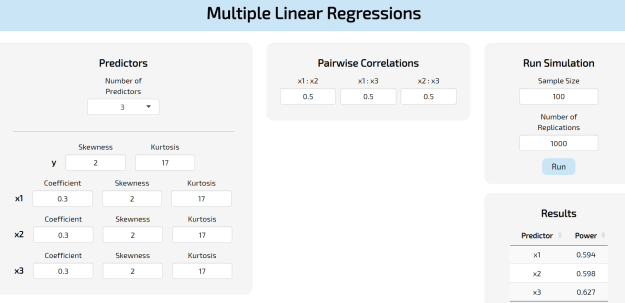
So the output under Results is the empirical, simulated power for each regression coefficient at the sample size selected. In this case, they gravitate around 60%.
Oh! And if for whatever reason you would like to have all your predictors be normal, you can set the values of skewness and kurtosis to 0. In fact, in that situation you would end up working with a multivariate normal distribution.
