So… here’s a trick I use sometimes that I’ve never seen anywhere else and it may be helpful to some people.

If you work with latent variable models, Factor Analysis, Structural Equation Modelling, Item Response Theory, etc. there’s a good chance that you have either encountered or have seen some version of a warning about a covariance matrix being “non positive definite”. This is an important warning because the software is telling you that your covariance matrix is not a valid covariance matrix and, therefore, your analysis is suspect. Usually, within the world of latent variables we call these types of warnings Heywood cases .

Now, most Heywood cases are very easy to spot because they pertain to one of two broad classes: negative variances or correlations greater than 1. When you inspect your matrix models and see either of those two cases, you know exactly which variable is giving you trouble. Thing is (as I found out a few years ago), there are other types of Heywood cases that are a lot more difficult to diagnose. Consider the following matrix that I once got helping a student with his analysis:


............space    lstnng    actvts    prntst    persnl    intrct    prgrmm
space       1.000
lstnng      0.599    1.000
actvts      0.706    0.646     1.000
prntst      0.702    0.459     0.653      1.000
persnl      0.591    0.582     0.844      0.776     1.00
intrct      0.627    0.964     0.501      0.325     0.639    1.000
prgrmm      0.493    0.602     0.981      0.687     0.944    0.642      1.000


This is the model-implied correlation matrix I obtained through the analysis which gave a Heywood case warning. The student was a bit puzzled because, although we had reviewed this type of situations in class, we had only mentioned the case of negative variances or correlations greater than one. Here he neither had a negative variance nor a correlation greater than one… but he still got a warning for non-positive definiteness.

My first reaction was, obviously, to check the eigenvalues of the matrix and, lo and behold, there it was:
[1] 5.01377877 1.00744933 0.62602056 0.30393170 0.16671742 0.01317704 -0.13107483

So… yeah. This was, indeed, an invalid correlation/covariance matrix and we needed to further diagnose where the problem was coming from… but how? Enter our good friend, linear algebra.

If you have ever taken a class in linear algebra beyond what’s required in a traditional methodology/statistics course sequence for social sciences, you may have encountered something called the minor of a matrix. Minors are important because they’re used to calculate the determinant of a matrix. They’re also important for cases like this one because they break down the structure of a matrix into simpler components that can be analyzed. Way in the back of my mind I remembered from my undergraduate years that positive-definite matrices had something special about their minors. So when I came home I went through my old, OLD notes and found this beautiful theorem known as Sylvester’s criterion:

A Hermitian matrix is positive-definite if and only if  all of the leading principal minors have positive determinant.

All covariance matrices are Hermitian (the subject for another blogpost) so we’re only left to wonder what is a principal minor. Well, if you imagine starting at the [1,1] coordinate of a matrix (so really the upper-left entry) and going downwards diagonally expanding one row and column at a time you’d end up with the principal minors. A picture makes a lot more sense for this:

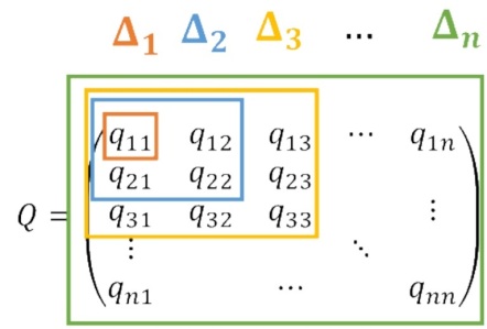
So… yeah. The red square (so the q11 entry) is the first principal minor. The blue square (a 2 x 2 matrix) is the 2nd principal minor, the yellow square (a 3 x 3 matrix) is the 3rd principal minor and on it goes until you get the full n x n matrix. For the matrix Q to be positive-definite, all the n-1 principal minors need to have positive determinant. So if you want to “diagnose” your matrix for positive definiteness, all you need to do is start from the upper-left corner and check the determinants consecutively until you found one that is less than 0. Let’s start from the previous example. Notice that I’m calling the matrix ‘Q’:
1
> det(Q[1:2,1:2])
[1] 0.641199
> det(Q[1:3,1:3])
[1] 0.2933427
> det(Q[1:4,1:4])
[1] 0.01973229
> det(Q[1:5,1:5])
[1] 0.003930676
> det(Q[1:6,1:6])
[1] -0.003353769


The first [1,1] corner is a given (it’s a correlation matrix so it’s 1 and it’s positive). Then we move downwards the 2×2 matrix, the 3×3 matrix… all the way to the 5×5 matrix. By then the determinant of Q is very small so I suspected that whatever the issue might be, it had to do with the relationship of the variables  “persnl”,  “intrct” or “prgrmm”. The final determinant pointed towards the culprit. Whatever problem this matrix exhibited, it had to do with the relationship between “intrct” and”prgrmm”.

Once I pointed out to the student that I suspected the problem was coming from either one of these two variables, a careful examination revealed the cause: The “intrct” item was a reverse-coded item but, for some reason, several of the participants respondents were not reverse-coded. So you had a good chunk of the responses to this item pointing to one direction and a smaller (albeit still large) number pointing to the other direction. The moment this item was full reverse-coded the non-positive definite issue disappeared.

I guess there are two lessons to this story: (1) Rely on the natural structure of things to diagnose problems and (2) Learn lots of linear algebra 🙂