::UPDATE::

A published article introducing this app is now online in BMC-Medical Research Methodology. If you plan on using this app, it would be a good idea to cite it 😉

The relationship between statistical power and predictor distribution in multilevel logistic regression: a simulation-based approach

 

WARNING (1): This app can take a little while to run. Do not close your web browser unless it gives you an error. If it appears ‘stuck’ but you haven’t got an error it means the simulation is still running on the background.

WARNING (2): If you keep getting a ‘disconnected  from server’ error, close down your browser and open a new window. If the problem still persists that means too many people have tried to access it during the day and the server has shut down. This app is hosted on a free server and it can only accommodate a certain number of people every day.  

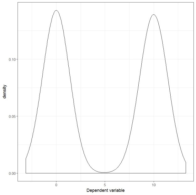
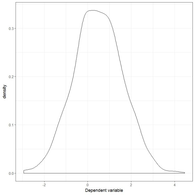
This app will perform computer simulations to estimate power for multilevel logistic regression models allowing for continuous or categorical covariates/predictors and their interaction. The continuous predictors come in two types: normally distributed or skewed (i.e. χ²  with 1 degree of freedom). It currently only supports binary categorical covariates/predictors (i.e. Bernoulli-distributed) but with the option to manipulate the probability parameter p to simulate imbalance of the groups.

The app will give you the power for each individual covariate/predictor  AND the variance component for the intercept (if you choose to fit a random-intercept model) or the slope (if you choose to fit a model with both a random intercept and a random slope). It uses the Wald test statistic for the fixed effect predictors and a 1-degree-of-freedom likelihood-ratio test for the random effects (← yes, I know this is conservative but it’s the fastest one to implement).

When you open the app, here’s how it looks:

What **you**, as the user, need to provide is the following:

The Level 1 and Level 2 sample sizes. If I were to use the ubiquitous example of “children in schools” the Level 1 sample would be the children (individuals within a cluster) and the Level 2 sample would be the schools  (number of clusters). For demonstration purposes here I’m asking for groups of 50 ‘children’ in 10 ‘schools’ for a total sample size of 50×10 = 500 children.

The variance for the random effects. You can either choose to fit an intercept-only model (so no variance of the slope) or a random intercept AND random slope model. You cannot fit a random-slope only model here and you cannot set the variances at 0 to fit a single-level logistic regression (there’s other software to do power analysis for single-level logistic regression). At least the variance of the intercept needs to be specified. Notice that the app defaults to an intercept-only model and under ‘Select Covariate’ it will say ‘None’. That changes when you click on the drop-down menu where it gives you the option of which random slope do you want. Notice that you can only choose one predictor to have a random slope. Will work on the general case in the future.

The number of covariates (or predictors) which I believe is pretty self-explanatory. Just notice that the more covariates you add, the longer it will take for the simulation to run. The default in the app is 2 covariates.

This would be the core of the simulation engine because the user needs to specify:

• Regression coefficients (‘Beta’).  This space lets the user specify the effect size for the regression coefficients under investigation. The default is 0.5 but that can be changed to any number. In the absence of any outside guidance, Cohen’s small-medium-large effect sizes are recommended. Remember that the regression coefficient for binary predictors is conceptualized as a standardized mean difference so it should be in Cohen’s d metric.
• Level of the predictor (‘Level’). It only supports 2-level models so the options are ‘1’ or ‘2’. This section indicates whether a predictor belongs to the Level 1 sample (e.g. the ‘children’) or the Level 2 sample (e.g. the ‘school). Notice that whichever predictor gets assigned a random slope MUST also be selected as Level 1. Otherwise the power analysis results will not make sense. It currently only supports one predictor at the Level 1 with a random slope. Other predictors can be included at Level 1 but they won’t have the option for a random slope component.
• Distribution of the covariates (‘Distribution’).  Offers 3 options: normally-distributed, skewed  (i.e. χ²  with 1 degree of freedom or a skew of about √8) and binary/Bernoulli-distributed. For the binary predictor the user can change the population parameter p and create imbalance between the groups. So, for instance, if p=0.3 then 30% of the sample would belong to the group labelled as ‘1’ and 70% to the group labelled as ‘0’. The default for this option is 0.5 to create an even 50/50 split.
• Intercept (‘Intercept Beta’).  Lets the user define the intercept for the regression model. The default is 0 and I wouldn’t recommend changing it unless you’re making inferences about the intercept of the regression model.

Once the number of covariates has been selected, the app will offer the user all possible 2-way interaction effects irrespective of the level of the predictor and distribution characteristics. The user can select whichever 2-way interaction is of interest and assign an effect size/regression coefficient (i.e. ‘Beta’). The app will use this effect size to calculate power. Notice that the distribution of the interaction is fully defined by the distribution of its constituting main effects.

The number of datasets generated using the population parameters previously defined by the researcher. The default is 10 but I would personally recommend a minimum of 100. The larger the number of replications the more accurate the results will be but also the longer the simulation will take.

The simulated power is calculated as the proportion of statistically significant results out of the number of simulated datasets and will be printed here. Notice the time progress bar indicating that the simulation is still running. For a 2-covariate model with both a random effect for the intercept and the slope the simulation took almost 3 min to run. Expect longer waiting times if the model has lots of covariates.

This is what a sample of a full power analysis looks like. The estimated power can be found under the column ‘Power’. The column labelled ‘NA’ shows the proportion of models that did not converge. In this case, all models converged (there are 0s all throughout the NA column) but the power of the fixed and random effects is relatively low with the exception of the power for the variance of the random intercept. In this example one would need to either increase the effect size from 0.5 to something larger or increase the Level 1 and Level 2 sample sizes in order to obtain acceptable power levels of 80%. You can either download your power analysis results as a .csv file or copy-paste them by clicking on the appropriate button.

Finally, here is the link for the shiny web app:

YOU CAN CLICK HERE TO ACCESS THE APP

 

If you’re an R user and would either like to see the code that runs underneath or would prefer to work directly with it for your simulation, you can check it out on my github account.

If this app is of any use to you and you’d like to cite it, please also cite the lme4, simglm and paramtest R packages. This is really just a shiny wrapper for the 3 packages put together. Those 3 packages are the ones doing most of the “heavy-lifting” when it comes to the simulation and calculations.

This shiny app will:

– Give you the polychoric (or tetrachoric, in case of binary data) correlation matrix

– Do Parallel Analysis and a scree plot based on the polychoric (or tetrachoric) correlation matrix

– Calculate ordinal alpha as recommended in:

Zumbo, B. D., Gadermann, A. M., & Zeisser, C.. (2007). Ordinal Versions of Coefficients Alpha and Theta For Likert Rating Scales. Journal of Modern Applied Statistical Methods, 6, 21-29.

It currently takes in certain SPSS files (so .sav file extensions from older versions of SPSS, say around 2013 or less), Microsoft Excel files (so .xls file extensions) and comma-delimited files (so .csv extensions). If your data is in none of those files, please change it before using the app (it’s super easy). or it will give you an error. Also notice that the app will use ALL of the variables in the file uploaded, so make sure you upload a file that only has the variables (test items in most cases) which you want to correlate/calculate alpha for. You’ll need to provide a clean dataset for it to work. So if you have missing values, you’ll need to manually remove them before submitting it. If there are outliers, those need to be dealt with before using the app.

Please notice that in accordance to research, if you have 8 (or more) Likert responses, the app will give you an error saying you have enough categories to safely treat your variables as continuous, so you don’t really need to use this app. You can see why in Rhemtulla, Brosseau-Liard & Savalei (2012).

YOU CAN CLICK HERE TO ACCESS THE APP

So… something interesting happened the other day. As part of an unrelated set of circumstances, my super awesome BFF Ed and I were discussing one of those interesting, perennial misconceptions within methodology in the social sciences. OK, maybe in other areas as well but I can only speak about what I know best. The interesting aspect of this conversation is that it reflects the differences in training that he and I have so that, although we tend to see things from the same perspective, our solutions are sometimes different. You see, Ed is a full-blown mathematician who specializes in harmonic analysis but with a keen interest in urban ornithology as his more “applied” researcher side. Oh, and some psychometrics as well. I’m a psychometrician that’s mostly interested in technical problems but also flirts with the analysis of developmental data. This is going to play an important role in how we approached the answer to the following question:

In a traditional ANOVA setting (fixed effects, fully-balanced groups, etc.)… Does one test the normality assumption on the residuals or the dependent variable?

Ed’s answer (as well as my talkstats.com friends): On the residuals. ALWAYS.

My answer: Although the distributional assumptions for these models is on the residuals, for most designs found in education or social sciences it doesn’t really matter whether you use the residuals or the dependent variable.

Who is right, and who is wrong? The good thing about Mathematics (and Statistics as a branch of Mathematics) is that there’s only one answer. So either he is right or I am. Here are the two takes to the answer with a rationale.

Ed is right.

This is a simplified version of his answer that was also suggested on talkstats. Consider the following independent-groups t-test as shown in this snippet of R code. I’m assuming if you’re reading this you know that a t-test can be run as a linear regression.


dv1 <- rnorm(1000, 10, 1)
dv2 <- rnorm(1000, 0, 1)
dv <- c(dv1, dv2)
g <- as.factor(rep(c(1,0), each=1000))

dat<-data.frame(dv,g)

res <- as.data.frame(resid(lm(dv~g)))
colnames(res)<-c("residual")

If you plot the dependent variable, it looks like this:

And if you plot the residuals, they look like this:

Clearly, the dependent variable is not normally distributed. It is bimodal, better described as a 50/50 Gaussian mixture if you wish. However, the residuals are very much bell-shaped and.. well, for lack of a better word, normally distributed. If we wanted to look at it more formally, we can conduct a Shapiro-Wilks test and see that it is not statistically significant.


shapiro.test(res$residual)
Shapiro-Wilk normality test
data: res$residual
W = 0.99901, p-value = 0.3432

So… yeah. Testing the dependent variable would’ve led someone to (erroneously) conclude that the assumption of normality was being violated and maybe this person would’ve ended up going down the rabbit hole of non-parametric regression methods… which are not bad per se, but I realize that for people with little training in statistics, these methods can be quite problematic to interpret. So Ed is right and I am wrong.

I am right.

When this example was put forward I pointed out to Ed (and other people involved in the discussion) to look at the assumption made regarding the population effect size. That’s a Cohen’s d of 10! Let’s see what happens when you run what’s considered a “large” effect size within the social sciences. Actually, let’s be very, very, VERY generous and jump straight from a Cohen’s d of 0.8 (large effect size) to a Cohen’s d of 1 (super large effect size?).

The plot of the dependent variable now looks like this:

And the residual plot looks like this:

Uhm… both the dependent variable and the residuals are looking very normal to me. What if we test them using the Shapiro-Wilks test?

shapiro.test(res$residual)
Shapiro-Wilk normality test

data: res$residual
W = 0.99926, p-value = 0.6328

shapiro.test(dv)
Shapiro-Wilk normality test

data: dv
W = 0.99944, p-value = 0.8515

Yup, both are pretty normal-looking. So, in this case, whether you test the dependent variable or the residuals you end up with the same answer.

Just for kicks and giggles, I noticed that you needed a Cohen’s d of 2 before the Shapiro-Wilks test yielded a significant result, but you can see that the W statistics are quite similar between the previous case and this one.  And we’re talking about sample sizes of 2000. Heck, even the plot of the dependent variable is looking pretty bell-shaped

shapiro.test(dv)
Shapiro-Wilk normality test

data: dv
W = 0.99644, p-value = 8.008e-07

This is why I, in my response, I included the addendum of for most designs found in education or social sciences it doesn’t really matter whether you use the residuals or the dependent variable. A Cohen’s d of 2 is two-and-a-half units larger than what’s considered a large effect size in my field. If I were to see such a large effect size, I’d probably think something funky going on with the data than actually believing that such a large difference can be found. Ed, comes from a natural science background. And I know that, in the natural sciences, large effect sizes are pretty common-place (in my opinion it comes down to the problem of measurement that we face in the social sciences).

As you can see now, the degree of agreement between the normality tests of the dependent variable and the residuals is a function of the effect size. The larger the effect size, the larger the difference between the shapes of the distributions of the residuals VS the dependent variable (within this context, of course. This is not true in general).

Strictly speaking, Ed and the talkstats team are right in the sense that you can never go wrong with testing the residuals. Which is what I pointed out in the beginning as well. My applied research experience, however, has made me more practical and I realize that, in most cases, it doesn’t really matter. And at a certain sample size, the normality assumption is just so irrelevant that even testing it may be unnecessary. But anyway, some food for thought right there 😉