So… something interesting happened the other day. As part of an unrelated set of circumstances, my super awesome BFF Ed and I were discussing one of those interesting, perennial misconceptions within methodology in the social sciences. OK, maybe in other areas as well but I can only speak about what I know best. The interesting aspect of this conversation is that it reflects the differences in training that he and I have so that, although we tend to see things from the same perspective, our solutions are sometimes different. You see, Ed is a full-blown mathematician who specializes in harmonic analysis but with a keen interest in urban ornithology as his more “applied” researcher side. Oh, and some psychometrics as well. I’m a psychometrician that’s mostly interested in technical problems but also flirts with the analysis of developmental data. This is going to play an important role in how we approached the answer to the following question:

In a traditional ANOVA setting (fixed effects, fully-balanced groups, etc.)… Does one test the normality assumption on the residuals or the dependent variable?

Ed’s answer (as well as my talkstats.com friends): On the residuals. ALWAYS.

My answer: Although the distributional assumptions for these models is on the residuals, for most designs found in education or social sciences it doesn’t really matter whether you use the residuals or the dependent variable.

Who is right, and who is wrong? The good thing about Mathematics (and Statistics as a branch of Mathematics) is that there’s only one answer. So either he is right or I am. Here are the two takes to the answer with a rationale.

Ed is right.

This is a simplified version of his answer that was also suggested on talkstats. Consider the following independent-groups t-test as shown in this snippet of R code. I’m assuming if you’re reading this you know that a t-test can be run as a linear regression.


dv1 <- rnorm(1000, 10, 1)
dv2 <- rnorm(1000, 0, 1)
dv <- c(dv1, dv2)
g <- as.factor(rep(c(1,0), each=1000))

dat<-data.frame(dv,g)

res <- as.data.frame(resid(lm(dv~g)))
colnames(res)<-c("residual")

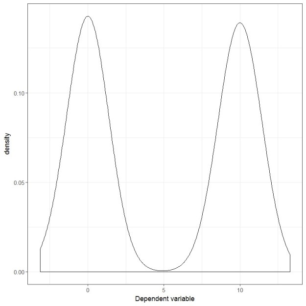
If you plot the dependent variable, it looks like this:

And if you plot the residuals, they look like this:

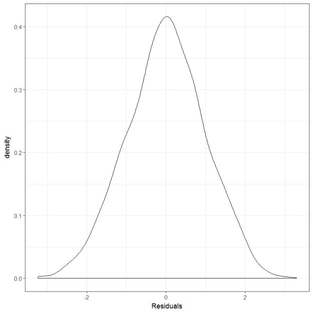
Clearly, the dependent variable is not normally distributed. It is bimodal, better described as a 50/50 Gaussian mixture if you wish. However, the residuals are very much bell-shaped and.. well, for lack of a better word, normally distributed. If we wanted to look at it more formally, we can conduct a Shapiro-Wilks test and see that it is not statistically significant.


shapiro.test(res$residual)
Shapiro-Wilk normality test
data: res$residual
W = 0.99901, p-value = 0.3432

So… yeah. Testing the dependent variable would’ve led someone to (erroneously) conclude that the assumption of normality was being violated and maybe this person would’ve ended up going down the rabbit hole of non-parametric regression methods… which are not bad per se, but I realize that for people with little training in statistics, these methods can be quite problematic to interpret. So Ed is right and I am wrong.

I am right.

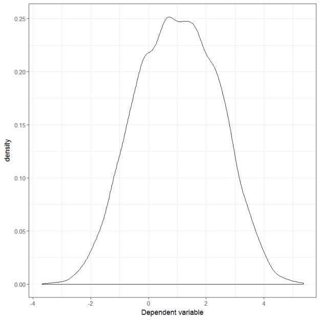
When this example was put forward I pointed out to Ed (and other people involved in the discussion) to look at the assumption made regarding the population effect size. That’s a Cohen’s d of 10! Let’s see what happens when you run what’s considered a “large” effect size within the social sciences. Actually, let’s be very, very, VERY generous and jump straight from a Cohen’s d of 0.8 (large effect size) to a Cohen’s d of 1 (super large effect size?).

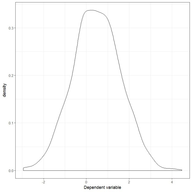
The plot of the dependent variable now looks like this:

And the residual plot looks like this:

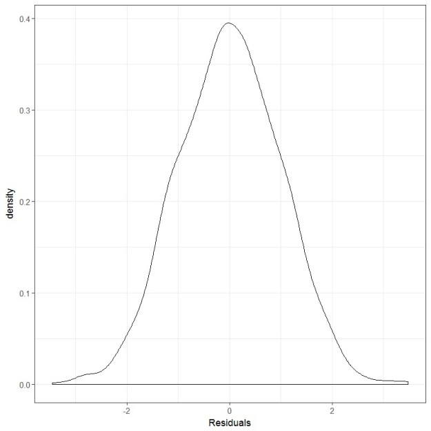
Uhm… both the dependent variable and the residuals are looking very normal to me. What if we test them using the Shapiro-Wilks test?

shapiro.test(res$residual)
Shapiro-Wilk normality test

data: res$residual
W = 0.99926, p-value = 0.6328

shapiro.test(dv)
Shapiro-Wilk normality test

data: dv
W = 0.99944, p-value = 0.8515

Yup, both are pretty normal-looking. So, in this case, whether you test the dependent variable or the residuals you end up with the same answer.

Just for kicks and giggles, I noticed that you needed a Cohen’s d of 2 before the Shapiro-Wilks test yielded a significant result, but you can see that the W statistics are quite similar between the previous case and this one.  And we’re talking about sample sizes of 2000. Heck, even the plot of the dependent variable is looking pretty bell-shaped

shapiro.test(dv)
Shapiro-Wilk normality test

data: dv
W = 0.99644, p-value = 8.008e-07

This is why I, in my response, I included the addendum of for most designs found in education or social sciences it doesn’t really matter whether you use the residuals or the dependent variable. A Cohen’s d of 2 is two-and-a-half units larger than what’s considered a large effect size in my field. If I were to see such a large effect size, I’d probably think something funky going on with the data than actually believing that such a large difference can be found. Ed, comes from a natural science background. And I know that, in the natural sciences, large effect sizes are pretty common-place (in my opinion it comes down to the problem of measurement that we face in the social sciences).

As you can see now, the degree of agreement between the normality tests of the dependent variable and the residuals is a function of the effect size. The larger the effect size, the larger the difference between the shapes of the distributions of the residuals VS the dependent variable (within this context, of course. This is not true in general).

Strictly speaking, Ed and the talkstats team are right in the sense that you can never go wrong with testing the residuals. Which is what I pointed out in the beginning as well. My applied research experience, however, has made me more practical and I realize that, in most cases, it doesn’t really matter. And at a certain sample size, the normality assumption is just so irrelevant that even testing it may be unnecessary. But anyway, some food for thought right there 😉