A while ago, a good friend of mine emailed me asking a very interesting question regarding how can you obtain the R-squared for an OLS multiple regression equation model simply from the correlation matrix of the predictors (and the criterion). He showed me a formula and I explained how said formula can be derived from some basic matrix operations on the correlation matrix. Another friend share with him the formulas from Cohen, Cohen, Aiken & West (Chp. 3 page 68) that relate the correlation matrix to the standardized regression coefficients and these to the R-squared. Nevertheless, my dear friend made a very good observation regarding both my solution and the other one:
Well like I said, it’s all very useful, but if I’m being nitpicky I don’t really consider either method to be “from scratch” for my purposes, since the first method relies on knowing the matrix expression in the first place, which I don’t know how to derive, and the second method relies on knowing those equations which I also don’t know how to derive.
Days became weeks, weeks became months and the problem was pretty much forgotten… until now. While I was working on a completely unrelated problem, I ended up finding exactly how to obtain the formulas from the Cohen et.al. book starting from the basic definition of the least-squares estimator for the regression coefficients. Cohen (being his usual Cohen self) merely provides the rather cryptic note (on p. 68) that “The equations for 


If you’re confused as far as where that comes from then the rest of this post won’t make sense so you can probably stop reading now. Nevertheless, I think any quantitative analyst worth his or her salt should be able to recognize the above equation and know exactly where it comes from. When the ineffable Cohen talks about “differential calculus” he is referring to that thing. Seriously, any book on linear algebra or regression (from a Math/Stats perspective) explains how to obtain it so I am just gonna assume that you know.
What many people may not know, however, is that the above expression is equivalent to:

Where 


An example using the ubiquitous dataset mtcars
lm(mpg ~ cyl + disp, data=mtcars)
Call:

lm(formula = mpg ~ cyl + disp, data = mtcars)
Coefficients:

(Intercept) cyl disp

34.66099 -1.58728 -0.02058
#this part takes out the predictors 'cyl' and 'disp' and the dependent variable 'mpg'

x1 <- mtcars$cyl

x2 <- mtcars$disp

y <- mtcars$mpg
#covariance matrix of the predictors

covX <- cov(mtcars[,2:3])
#vector with the covariances of each predictor and the dependent variable

cov_xy <- c(cov(x1,y), cov(x2,y))
#least-squares solution to obtain the regression coefficients
solve(covX)%*%cov_xy
[,1]
cyl -1.58727681
disp -0.02058363
#this matches exactly what we had above for the regression coefficients using the lm() function
Now, why does this happen? Well, if you know a little bit of matrix algebra (particularly its relationship with statistics and the general linear model more specifically) you’ll know that 
Xc <- as.matrix(scale(mtcars[,2:3], scale=F)) #centers the predictors
(t(Xc)%*%Xc)*(1/(32-1)) #this 1/(32-1) is the correction factor for the sample size/dfs
cyl disp

cyl 3.189516 199.6603

disp 199.660282 15360.7998
#and this gives you the same result as
> cov(mtcars[,2:3])
cyl disp
cyl 3.189516 199.6603
disp 199.660282 15360.7998
So now we know that:

Because they’re both doing the same algebraic operations on the data. The degrees of freedom cancel out because the inverse function of the matrix, when applied to a constant, turns it into 1/constant and the vector of covariances between the predictors and the dependent variable are themselves being divided by the degrees of freedom, so you’re going to end up with a factor of

In a similar fashion (and this is where the Cohen et.al. formulas are gonna come in) if you want the standardized regression coefficients you would work with standardized covariances, which are better known as correlations. In this case, the formula is simply:

Where 

If we were to express this in full matrix form (and following the Cohen et.al. notation) we would have:
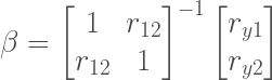
Where 


You can either invert this matrix and do the multiplications by hand (I’ll let you do that) or you can use a CAS (Computer Algebra System) to do it for you. I work with Maple so I did the necessary matrix operations there and what came out from it was:

Looks familiar? I’m sure it does! All that is missing is simplify it further (the term outside the vector is a constant so it multiplies each entry inside of it), and factor out a -1/-1 from the numerator and denominator to end up with:


Which are the exact formulas that you would find in the Cohen et.al. regression book on page 68.
Well, now that we’ve derived those formulas the final question (and the main purpose of this post) is to explain how this is all related to R-squared. Deriving the expression for R-squared as Cohen et.al. show requires a lot of terribly boring algebra and very careful book-keeping of the indices of each correlation… which is something I’m not interested in doing right now ;). I will only show the answer I provided (which I stole from Wikipedia because (a) I like it better since *I* suggested it 😀 and (b) the final step gives you an insight into where the actual formula from the Cohen et.al. text book comes from. My solution requires a tad bit more linear algebra so if you don’t really know much about it you’re probably gonna get lost. Just take my word for it then, I know what I’m doing…most of the time XD.
Anyhoo, the key here is to work solely in terms of standardized variables. We will use Z to denote that the variables are standardized and a sub-script to see to which variable it corresponds. In terms of matrix algebra, the standardized OLS regression model looks like:

Where 


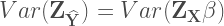

Now, remember that we derived 

Because 

And from here we obtain the Wikipedia formula that I suggested as an answer:

Moreover, using again the definition of the standardized regression coefficients in terms of the correlations among the variables, you can see that:

And here is where the Cohen et.al.’s formula on page #70 comes from. If you know the rules of matrix multiplication you can readily see that this matrix product is algebraically equivalent to what Cohen et. al. wants you to do to obtain the R-squared.
One less mathematical mystery unraveled by yours truly 🙂
