I think to honour one of my very first posts on this page, it would be nice to tackle the rather mild problem of how to simulate data that with a population value of Cronbach’s alpha. It’s a straightforward enough case that it won’t make me sweat 😛 and I will show both the latent-variable/SEM approach VS the traditional covariance matrix approach.
From a Covariance Matrix approach
As we know already, for Cronbach’s Alpha to be an unbiased estimate of the reliability of a scale, said scale needs to follow either a parallel-test model or a tau-equivalent model. Now, how does this translate into a population covariance matrix of items? Well, interestingly enough there are two covariance structures (with funky names, actually) implied by them. The first one is pretty well known: compound symmetry. That is correct, boys and girls. IF one assumes a one-factor model in the population a compound-symmetric covariance matrix would imply the parallel-test model holds. The second one I have only found in the SPSS manual so I will use its name: heterogeneous compound symmetry. Which basically just implies that the variances of the variables (items, in this case) can be different but their covariances must be the same. I don’t know if heterogeneous compound symmetry is a ‘thing’ or not, but heck. I’ll stick with it.
In any case, so why does this matter? Well, because if we know what the covariance structure that we want looks like, we can just plug that in our friendly R and get data the way we like it, yo! Here, I will rely on the correlation matrix to simulate a standardized alpha (so the distinction between compound and heterogneous compound symmetry gets blurred) and will simply use this hand-dandy Wiki formula:
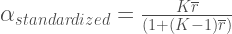
Where K is the number of variables (items) and 
So, on to R now. Say I want an alpha of 0.8 in the population. After a little bit of trial and error I saw that a 4-item scale with population correlations of 0.5, would give me standardized alpha of 0.8. So I literally just did:
library(MASS)

library(psych)
Sigma <- matrix( c(1, .5, .5, .5,

.5, 1, .5, .5,

.5, .5, 1, .5,

.5, .5, .5, 1), 4,4)
N <- 100
datam <- as.data.frame(mvrnorm(100, c(rep(0,4)), Sigma))
alpha(datam)
As you can see, eve at a sample size of N=100 you’re already getting estimates pretty close to the population estimate.
From a Structural Equation Modeling approach.
Anyone who simulates data with specified values of reliability doesn’t usually do so from a covariance-matrix only standpoint. The more modern way to go about this is by specifying a SEM model and by conveniently choosing the loadings and the error variances, One can create any covariance structure that one likes. Under the one-factor model (which is needed for Cronbach’s Alpha to be an accurate estimate), the covariance matrix of your data would look something like this:
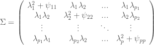
Or, in other words all the covariances are products of the loadings of the items and the variances are the loadings squared plus some error variance. For the tau-equivalent/parallel test model to hold, the loadings have to be equal in the population across items. The formula for the reliability of the scale works almost the same as the reliability of alpha, which is the variance attributed to the factor (so the sum of the loadings squared) divided by the total variance (so the sum of the loadings squared + the error variances). It’ll be a lot easier to see with an example.
In this case, the name of the game is to simply choose my loadings to reflect the alpha that I want in the population. Borrowing from the example above, which number, when multiplied times itself gives me 0.5 (or something close to 0.5)? Well… 0.7 would be the closest. So all I need to do is build a one factor model with 4 indicators where all the loadigs are 0.7 and that would give me a population alpha of 0.8. I’ll use the lavaan package to help me along
library(psych)

library(lavaan)
mod1 <- 'f1=~ .7*x1 + .7*x2 + .7*x3 + .7*x4'
datum <- simulateData(mod1, sample.nobs=1000, standardized=TRUE)
alpha(datum)
And, as you can see when you plug this in R, alpha is, once again, 0.8!
