Being in quarantine helps one catch up with a few unfinished projects. One of them was for me to re-read Chapter 4 of one of the classic of classics of psychometrics: Nunnally & Bernstein’s Psychometric Theory  This is one of those must-have psychometrics textbooks because of the impact it has had on the field. You see it cited everywhere and with more than 124,000 citations and counting (as per Google Scholar), it’s not surprising. Remember the magic threshold of Cronbach’s alpha>0.7 as acceptable reliability? Yup, that’s where you’d find it. Interestingly enough, the reason of why I wanted to re-read Chapter 4 was not necessarily to become re-acquainted with an important psychometric textbook. It’s because I remember reading claims there that were…well… let’s just call them less-than-ideal ;).

The problem with finding less-than-ideal claims in such a prominent text is that (much like with a virus), multiple copies of those claims get replicated and the “wrongness” just keeps spreading the more they get cited. What got me into reading it again was this article of mine that touches on Chapter 4 of Nunnally & Bernstein. At first I read it in passing and had to put the proverbial pin on it because life gets busy and things need to get done. But I am not as busy anymore, so I was able to re-read it to verify my suspicion of whether or not what I read meant what I thought it meant. And it did. These claims are all related to the Pearson correlation coefficient and the interplay between this statistic and the distributional shape of the variables. The first collection of claims can be found on page #132:

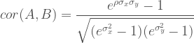
Let’s begin with the first claim: The most obvious example is that one cannot obtain a perfect correlation between two variables unless they have exactly the same distribution form. What Nunnally & Bernstein are alluding to in some indirect way is an old (but very useful) result from Copula Distribution Theory known as the Fréchet–Hoeffding bounds. What the Wiki essentially says is that for a bivariate distribution (we’ll only talk about bivariate distribuions here), the shape of its one-dimensional marginals places undue bounds on the Pearson correlation coefficient. Therefore, depending on what gets correlated with what, the correlation coefficient’s theoretical lower and upper bounds will not be -1 or +1. They’ll be something smaller (in absolute value).

The easiest counterexample to the first claim comes from joint-distributions with log-normal marginals. I go into more detail about this in this other blog post of mine, because the log-normal distribution has a very amenable form to calculate its Fréchet-Hoeffding bounds. You can get all the mathematical details in all its gory glory in Appendix A of this article but, essentially, consider a bivariate normal distribution with non-zero correlation coefficient , standard deviations and   (<— this just make the derivation simpler and the take-home message is the same). Now define so that now are each log-normally distributed. The new correlation coefficient between the two log-normal random variables is now:

Let’s take a very simple example and pretend both are standardized so that and . If you do the appropriate substitutions above and set for the maximum and for the minimum, then it becomes easy to see that:

Just for reference . So here we are taking Nunnally & Bernstein’s claim and take it to the extreme. Not only do both variables have the same distributional shape, they even have the same parameters. And the correlation coefficient still doesn’t span the [-1, +1] range.

In the same page they continue:

Let’s start with the second claim: (2) how different in shape the distributions are. This is a tad bit ambiguous to me because what exactly does “different” mean here? Consider the case of a joint distribution where one marginal is and the other is .  The joint distribution would look something like this:

And a good, empirical approximation to the Fréchet–Hoeffding bounds can be obtained in R through simulation (because y’all know that simulation’s mah thang 🙂 ):

a<-runif(1000000, min=0, max=1)
b<-rbeta(1000000, shape1=2, shape2=2)
cor(sort(a),sort(b))
[1] 0.9959238

Are those distributions “different” enough? I mean, one has a peak at its centre and fast-decreasing tails. The other has no peak and no tails. Yes, I am aware that a beta distribution with equal shape parameters 1 is a uniform distribution. Well, let’s give the beta-distributed random variable very large shape parameters so it (approximately) converges to the normal and try the bounds again:

a<-runif(1000000, min=0, max=1)
b<-rbeta(1000000, shape1=200, shape2=200)
cor(sort(a),sort(b))
[1]0.9772489

There’s a difference of a little under 0.02 between the above maximum correlation and this one. Are those distributions different enough now? I think that, as it stands, this claim either needs more context or it is not entirely correct.

Let’s move on to the final claim: (1) how high the correlation would have been if the distributions had the same shape. This is also not entirely accurate because the size of the correlation does not play that big of a role in terms of how restricted the theoretical range can be. What is important are the forms of the cumulative density functions (CDFs) of the lower-dimensional marginal distributions. Consider Hoeffding’s covariance identity for two random variables. In “standard” copula notation:

where is the joint-CDF of the random variables and , is the marginal CDF of the random variable and is the marginal CDF of the random variable . The Fréchet–Hoeffding bounds are then:

The “classical” form of the bounds is in terms of the covariance, but standardizing them would give the bound for the correlation. Notice how the endpoints do not even reference it! They’re all in terms of the one-dimensional marginals. I’m going to use our friend the log-normal distribution again to make it easier. Consider . We know that if we were to do something like then because is just a scaled , right? Well, if you exponentiate both and to transform the normal distributions into log-normal distributions, then it’s not hard to show (it’s actually a well-known identity within the theory of log-normal distributions) that:

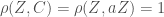
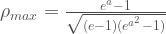
And that’s it. The maximum possible correlation depends entirely on what the value of is. It’s not super difficult to show in R. Compare the “base case”:


set.seed(123)
x<-rnorm(100000)
y<-1*x
a<-exp(x)
b<-exp(y)

> cor(sort(a), sort(b))
[1] 1

With a test case:
set.seed(123)
x<-rnorm(100000)
y<-2*x
a<-exp(x)
b<-exp(y)

> cor(sort(a), sort(b))
[1] 0.7514706

Yeah… quite a bit of shrinkage! The graph below shows how the maximum possible correlation decreases as the scaling factor increases. Which is kind of crazy if you think about it because by the time the scaling factor is 5, both random variables are perfectly dependent yet the Pearson correlation coefficient is (approx) 0.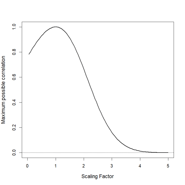

There are other claims within that Chapter that have made me raise my eyebrows more than once. But those need a little bit more formal analysis to show where the misconception may be. I think at the end of the day, when Nunnally & Bernstein say “exactly the same distribution” they were tacitly assuming the distributions should be symmetric and, ideally, both symmetric and unimodal. For some reason that I haven’t quite figured out yet, the Fréchet–Hoeffding bounds tend to span *almost* the full theoretical range [-1, +1] when both marginal distributions are symmetric and unimodal. I’ve actually had a hard time finding a case where the theoretical range is severely shrunk yet both distributions are symmetric and unimodal (no, the Cauchy distribution doesn’t count, sorry!). So…until then… Nunnally & Bernstein…NEEDS (a small) REVISION!