While I was cleaning up some files on my computer, I found an old homework problem set where I just casually wrote in one answer “it can be trivially shown that a Canonical Correlation analysis with only one dependent variable reduces to a Multiple Regression analysis”. Me being the scatter-minded student I was, never really bothered to show it. But now that I have a little bit more time to work on these things, I think it would be interesting to highlight some of the connections between univariate and multivariate versions of the General Linear Model and how things reduce naturally to traditional methods we all know and love when you jump back from multiple dimensions to one.
I’m assuming people who are reading this are familiar with both Multiple Regression and Canonical Correlation Analysis, but perhaps not with how they are connected. Now, at the core of Canonical Correlation Analysis are, of course, the pairs of Canonical Variates and their respective Canonical Correlations. Consider the case of two 


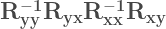
Where 


Compare that previous matrix to the one I used on my post about how the correlation matrix can be used to obtain the R-squared in Multiple Regression

Where 

Notice the similarities? In Multiple Regression we only have one vector-valued (*not* matrix-valued) variable 

library(MASS)

set.seed(123)
## creates some fake data

Sigma <- matrix(rep(0.5, 5^2),5,5)

diag(Sigma)<-1

mu <- rep(0,5)

dat <- as.data.frame(mvrnorm(1000,mu,Sigma))
## runs multiple regression and canonical correlation analyses

mod0 <- lm(V1 ~ V2 + V3 + V4 + V5, data=dat)

mod1<-cancor(dat[,2:5], dat[,1])
## the squared canonical correlation equals the multiple regression R-squared summary(mod0)$r.squared
[1] 0.4097961
> mod1$cor^2

[1] 0.4097961
Pretty cool, huh? Now, what about the coefficients? Well those are slightly trickier, You see, although the problems tackled by Canonical Correlation and Multiple Regressions are related they are not exactly the same. That’s why they scale their coefficients differently. For instance, have a look at how the Multiple Regression coefficients look compared to the Canonical Correlation ones:
> mod1$xcoef

[,1]        [,2]        [,3]        [,4]

V2 -0.009625799  0.031325139  0.017761087  0.015644448

V3 -0.013968658 -0.031445156  0.017423379  0.010808743

V4 -0.009153013  0.002859411 -0.037375716  0.008994849

V5 -0.007230093  0.002258689  0.001114241 -0.040591875
>mod0

Call:

lm(formula = V1 ~ V2 + V3 + V4 + V5, data = dat)
Coefficients:

(Intercept) V2 V3 V4 V5

0.008087 0.195300 0.283413 0.185708 0.146693
Yeah, not even close. But this really is just a matter of scaling more than anything else so, for the proper scaling constant, you can find the relationship between the Canonical Correlation coefficients (aka “loadings”) and the Multiple Regression ones. For this, a very useful package to use is the ‘matlib’ package and consider the set of of Canonical coefficients as linear equations related to the set of Multiple Regression ones. In more traditional linear algebra terms, solving for the equation 


library(matlib)

A<-mod1$xcoef

b<-coef(mod0)[-1]
> Solve(A, b, fractions=F)

x1        =  -20.289242

x2      =           0

x3    =           0

x4  =           0
So the constant -20.289242 relates the first set of $xcoef loadings from the Canonical Correlation Analysis to the Multiple regression coefficients. Just to verify:
### first set of Canonical coefficients

mod1$xcoef[,1]

V2           V3           V4           V5

-0.009625799 -0.013968658 -0.009153013 -0.007230093
### multiple regression (without the intercept) coefficients

coef(mod0)[-1]

V2        V3        V4        V5

0.1953002 0.2834135 0.1857077 0.1466931
###canonical correlation loadings scaled to match multiple regression

> mod1$xcoef[,1]*-20.289242

V2        V3        V4        V5

0.1953002 0.2834135 0.1857077 0.1466931
